Applied Mathematics
Vol.07 No.07(2016), Article ID:65822,11 pages
10.4236/am.2016.77056
A Compact Finite Difference Schemes for Solving the Coupled Nonlinear Schrodinger-Boussinesq Equations
M. S. Ismail, H. A. Ashi
Department of Math, College of Science, King Abdulaziz University, Jeddah, Saudi Arabia

Copyright © 2016 by authors and Scientific Research Publishing Inc.
This work is licensed under the Creative Commons Attribution International License (CC BY).
http://creativecommons.org/licenses/by/4.0/


Received 12 February 2016; accepted 22 April 2016; published 25 April 2016
ABSTRACT
In this paper we are going to derive two numerical methods for solving the coupled nonlinear Schrodinger-Boussinesq equation. The first method is a nonlinear implicit scheme of second order accuracy in both directions time and space; the scheme is unconditionally stable. The second scheme is a nonlinear implicit scheme of second order accuracy in time and fourth order accuracy in space direction. A generalized method is also derived where the previous schemes can be obtained by some special values of l. The proposed methods will produced a coupled nonlinear tridiagonal system which can be solved by fixed point method. The exact solutions and the conserved quantities for two different tests are used to display the robustness of the proposed schemes.
Keywords:
Coupled Nonlinear Schrodinger-Boussinesq Equation, Conserved Quantities, Soliton, Plane Wave Solution, Fixed Point Method

1. Introduction
In this work we are going to derive a highly a accurate schemes for the coupled nonlinear Schrödinger- Boussinesq equations (CSBE)
 (1)
(1)
 (2)
(2)
where ,
,  represents the complex short wave amplitude,
  represents the long wave amplitude,
  and
and  are real parameters. Equations (1) and (2) were considered as a model of the inter- actions between short and intermediate long waves, and were originated in describing the dynamics of Langmuir soliton formation, the interaction in plasma [1] - [4] . Numerical solution of coupled nonlinear Schrödinger equation using different methods can be found in [5] - [8] . Few numerical methods exist in literature for solving the CSBE. Zhang et al. [9] derived a conservative difference scheme to solve the CSBE. Bai et al. [1] [2] proposed the time splitting Fourier spectral method and the quadratic B-spline finite element method for solving the CSBE. Recently, a multi-symplectic scheme for solving the CSBE is developed in [10] .
2. Exact Solution
To derive the exact solution of the given system (1)-(2), we assume the solution of the CSBE of the form
 (3)
(3)
 (4)
(4)
where

By substituting (3) and (4) into (1) and (2), and after lengthy calculations, we found that the solution exists if we have the following relations
 (5)
(5)
where  and c are arbitrary constant.
The system (1)-(2) also has a plane wave solution
 (6)
(6)
where A, k, and d are constants.
3. Properties of the CSBE
In order to study the properties of the coupled nonlinear Schrödinger-Boussinesq equation, we consider the initial boundary value problem [1] [10]
 (7)
(7)

with the initial conditions
 (8)
(8)
and boundary conditions of the forms
 (9)
(9)
where  and
and  are given smooth functions and these functions can be extracted from the exact solution, and
 (10)
(10)
By introducing the function  such that
 (11)
(11)
and the boundary conditions
 (12)
(12)
the CSBE coupled system can be written as
 (13)
(13)
 (14)
(14)
 (15)
(15)
For the initial-boundary value problem (13)-(14), there are at least three conservation laws [10] .
1) The Langmuir Plasmon number
 (16)
(16)
2) The total perturbed number density
 (17)
(17)
3) The total energy
 (18)
(18)
Physically, these conserved laws play major roles in all physical theories, and can be useful tools for qualitative analysis. Trapezoidal rule and the numerical solution are used to calculate the conserved quantities. The conservation of the conserved quantities for the proposed system using the numerical methods presented in this work is a good indication for the efficiency and robustness these methods.
4. Numerical Methods
In order to avoid the complex computation [5] - [7] we assume
 (19)
(19)
so, the CSBE can be written as
 (20)
(20)
 (21)
(21)
 (22)
(22)
 (23)
(23)
where
 (24)
(24)
We will consider the numerical solution of the nonlinear system (20)-(23) in a finite interval  We assume
  where
where  and h is the space grid step size, also we assume
  where k is the time grid step size, we assume
  We denote the exact and numerical solutions at the grid point
  by
by  and
and , respectively.
4.1. Second Order Scheme
The Crank Nicolson like scheme for the system (20)-(23) can be displayed as follows
 (25)
(25)
 (26)
(26)
 (27)
(27)
 (28)
(28)
where

The scheme in (25)-(28) is a nonlinear implicit scheme with block nonlinear tridiagonal structure. The fixed point method is used to solve this system. The scheme is of second order accuracy in both direction space and time. The scheme is unconditionally stable using the von Neumann stability analysis.
4.2. Fourth Order Scheme
In order to improve the accuracy in space direction, we approximate the second space derivative using the compact approximation

by using this , we will can derive the highly accurate compact finite difference scheme
 (29)
(29)
 (30)
(30)
 (31)
(31)
 (32)
(32)
The scheme in (29)-(32) is a nonlinear implicit scheme of fourth order accuracy in space and second order in time. To obtain the numerical solution, we need to solve a block nonlinear tridiagonal system at each time step. We have done this by using fixed point method. Using von Neumann stability analysis the scheme is also unconditionally stable.
4.3. Generalized Finite Difference Scheme
In this subsection we present the generalized finite difference scheme of the form
 (33)
(33)
 (34)
(34)
 (35)
(35)
 (36)
(36)
where  is an arbitrary constant. The scheme (33)-(36) is of second order accuracy in time and space for all
values of  The scheme is unconditionally stable. It is very easy to see that for
  we will get the second order method (25)-(28), while
  produced the fourth order method (29)-(32). In the next
subsection we present a fixed point iterative scheme to solve the nonlinear system obtained.
5. Fixed Point Method
In order to get the numerical solution for the nonlinear system (33)-(36), we propose the following fixed point iterative scheme of the following form
 (37)
(37)
 (38)
(38)
 (39)
(39)
 (40)
(40)
where
 (41)
(41)
 and
and
 (42)
(42)
We apply the iterative scheme (37)-(40) until the following condition
 (43)
(43)
is satisfied. Tol is a very small prescribed value.
6. Accuracy of the Generalized Scheme
To study the accuracy of the proposed scheme, we will consider only Equation (33), the other equations can be analyzed in the similar fashion. By replacing the numerical solution  by the exact solution
  to get
 (44)
(44)
By using Taylor’s series expansions of all terms in Equation (44), we will end with the local truncation error (LTE)
 (45)
(45)
and this indicates that, the scheme is of second order accuracy in space and time directions for arbitrary
 It is very interesting to notice that for
  the local truncation will be reduced to the fourth order
accuracy in space and second order accuracy in time.
7. Conserved Quantities
To prove that the decomposed system
 (46)
(46)
 (47)
(47)
 (48)
(48)
satisfies the conserved quantities
 (49)
(49)
and
 (50)
(50)
we multiply Equation (46) and Equation (47) by  and
and  respectively to get
 (51)
(51)
 (52)
(52)
by adding (51) and (52), this will lead us after some manipulation to the following equation
 (53)
(53)
By integrating (53) with respect to x, we get
 (54)
(54)
By imposing the vanishing boundary conditions, Equation (54) will be reduced to
 (55)
(55)
which is Equation (49).
To prove the second conserved quantity , by integrating Equation (48) with respect to x and this will lead us to the following
 (56)
(56)
and by imposing the vanishing boundary conditions, this will lead us to the second conserved quantity (50).
To prove that the proposed schemes preserve the discrete analog of the invariant (49) and (50), we borrow the following lemma [8] [11] .
Lemma 1 For any two discrete functions  and
and
 there is the identity

where


We will only prove the Crank Nicolson (25)-(28).
 (57)
(57)
 (58)
(58)
we multiply (57) by  and (58) by
  and then by adding the resulting equations to obtain

or
 (59)
(59)
which is the discrete analog of the conserved quantity (49), this indicates that no blow up in the numerical solution, and it it is a good indication the scheme is unconditionally stable. The second discrete conserved quantity can be easily obtained.
8. Numerical Results
In this section , we will test the proposed schemes for two different problems. The infinity error norm is used to calculate the error, and this can be defined by


Trapezoidal rule is used to approximate the conserved quantities. We will present some numerical results for the solitary wave solutions and the plane wave solutions for the coupled Schrodinger-Boussinesq equations.
8.1. Solitary Wave Solution
In this test, we choose the initial conditions


where  We choose the set of parameters

In Table 1 and Table 2, we present the  error norms and the conserved quantities for second and fourth order schemes respectively. Both methods preserve the conserved quantities almost exactly. Figure 1 and Figure 2 display the numerical solution of the proposed system for
  Results in both tables show the superior performance of both schemes in solving numerically the CSBEs equation, though the fourth order outperform the second order method as it produces the most accurate solution.

Table 1.  error norms and the conserved quantities for Crank Nicolson method.
Table 2.  error norms and the conserved quantities for the fourth order method.
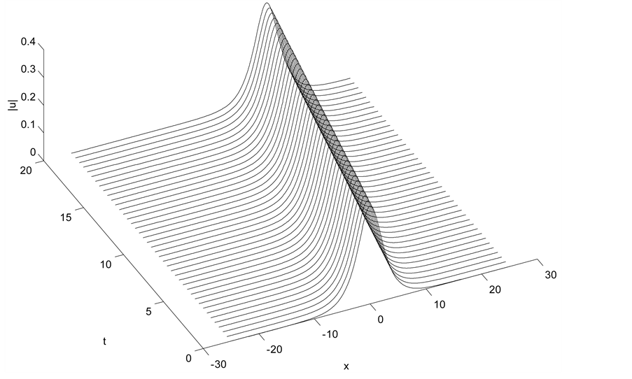
Figure 1. Single soliton: .
.
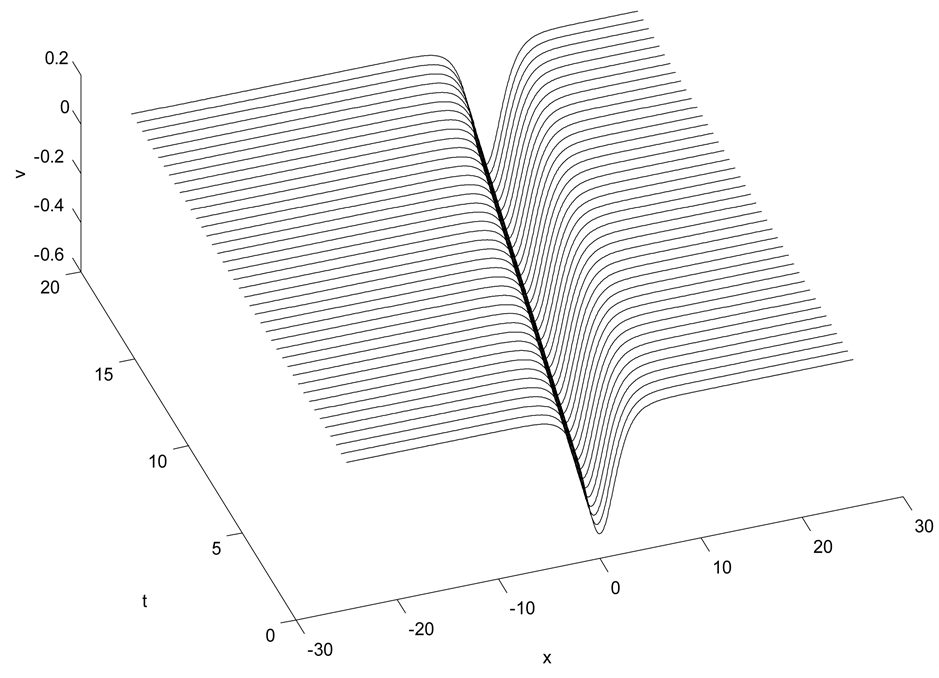
Figure 2. Single soliton: .
.
8.2. Plane Wave Solution
The initial conditions in this case are chosen as


In this test we select the set of parameters

together with the boundary conditions

The conserved quantities and the infinity error norm are given in Table 3 and Table 4 for second and fourth order numerical schemes respectively. The results show that the two schemes solve this problem exactly and conserve the conserved quantities exactly as well. In Figure 3, we display the modulus of the numerical solution of U at 
9. Conclusion
In this work, we transform the coupled Schrödinger-Boussinesq equations into a first order differential system in time. We derived two different numerical schemes. Using these methods, a coupled nonlinear block tridiagonal system is obtained. A fixed point iterative method is used to solve this system. The numerical tests and the conserved quantities show the efficiency and robustness of the schemes. To sum up, the proposed schemes are
Table 3. Crank Nicolson λ = 0 plane wave solution.
Table 4. Fourth order method with  plane wave solution.
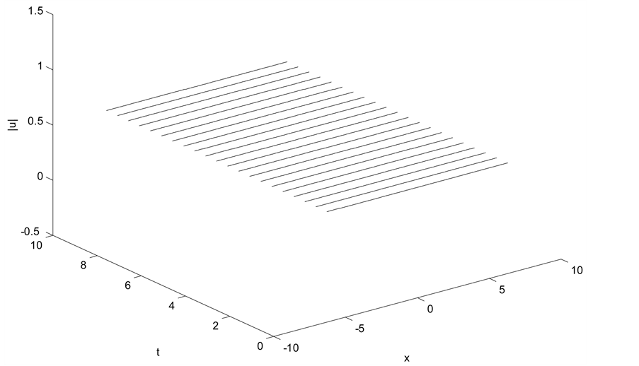
Figure 3. Plane wave solution with paraamters:  and d = 0.5.
reliable and capable to solve like systems.
Cite this paper
M. S. Ismail,H. A. Ashi, (2016) A Compact Finite Difference Schemes for Solving the Coupled Nonlinear Schrodinger-Boussinesq Equations. Applied Mathematics,07,605-615. doi: 10.4236/am.2016.77056
References
- 1. Bai, D. and Zhang, L. (2011) The Quadratic B-Spline Finite Element Method for the Coupled Schrödinger-Boussinesq Equations. International Journal of Computer Mathematics, 88, 1714-1729.
http://dx.doi.org/10.1080/00207160.2010.522234 - 2. Bai, D. and Wang, J. (2012) The Time-Splitting Fourier Spectral Method for the Coupled Schrödinger-Boussinesq Equations. Communications in Nonlinear Science and Numerical Simulation, 17, 1201-1210.
http://dx.doi.org/10.1016/j.cnsns.2011.08.012 - 3. Fan, E. (2000) Extended Tanh-Function Method and Its Applications to Nonlinear Equations. Physics Letters A, 277, 212-218.
http://dx.doi.org/10.1016/S0375-9601(00)00725-8 - 4. Fan, E. (2003) An Algebraic Method for Finding a Series of Exact Solutions to Integrable and Non-Integrable Nonlinear Evolution Equations. Journal of Mathematical Physics, 36, 7009-7026.
http://dx.doi.org/10.1088/0305-4470/36/25/308 - 5. Ismail, M.S. and Taha, T.R. (2001) Numerical Simulation of Coupled Nonlinear Schrödinger Equation. Mathematics and Computers in Simulation, 56, 547-562.
http://dx.doi.org/10.1016/S0378-4754(01)00324-X - 6. Ismail, M.S. and Alamri, S.Z. (2004) Highly Accurate Finite Difference Method for Coupled Nonlinear Schrödinger Equation. International Journal of Computer Mathematics, 81, 333-351.
http://dx.doi.org/10.1080/00207160410001661339 - 7. Ismail, M.S. and Taha, T.R. (2007) A Linearly Implicit Conservative Scheme for the Coupled Nonlinear Schrödinger Equation. Mathematics and Computers in Simulation, 74, 302-311.
http://dx.doi.org/10.1016/j.matcom.2006.10.020 - 8. Wang, T., Gue, B. and Zhang, L. (2010) New Conservative Schemes for Coupled Nonlinear Schrödinger System. Applied Mathematics and Computation, 217, 1604-1619.
http://dx.doi.org/10.1016/j.amc.2009.07.040 - 9. Zhang, L., Bai, D. and Wang, S. (2011) Numerical Analysis for a Conservative Difference Scheme to Solve the Schrödinger-Boussinesq Equation. JCAM, 235, 4899-4915.
- 10. Huang, L.Y., Jiao, Y.D. and Liang, D.-M. (2013) Multi-Symplectic Scheme for the Coupled Schrödinger Boussinesq Equations. Chinese Physics B, 22, 07020-1-07020-5.
- 11. Chang, Q., Jia, E. and Sun, W. (1999) Difference Schemes for Solving the Generalized Nonlinear Schrödinger Equation. Journal of Computational Physics, 148, 397-415.
http://dx.doi.org/10.1006/jcph.1998.6120