Applied Mathematics
Vol.5 No.7(2014), Article ID:44811,24 pages DOI:10.4236/am.2014.57101
Continued Fractions and Dynamics
Stefano Isola
Dipartimento di Matematica e Informatica, Università degli Studi di Camerino, Camerino Macerata, Italy
Email: stefano.isola@unicam.it
Copyright © 2014 by author and Scientific Research Publishing Inc.
This work is licensed under the Creative Commons Attribution International License (CC BY).
http://creativecommons.org/licenses/by/4.0/
![]()

Received 17 January 2014; revised 17 February 2014; accepted 24 February 2014
ABSTRACT
Several links between continued fractions and classical and less classical constructions in dynamical systems theory are presented and discussed.
Keywords:Continued Fractions, Fast and Slow Convergents, Irrational Rotations, Farey and Gauss Maps, Transfer Operator, Thermodynamic Formalism

1. Introduction
The connection between Number Theory and Dynamical Systems Theory is receiving recently a considerable attention. In this paper, we review some aspects of this connection focusing on the interplay between continued fractions and one dimensional dynamics. In Section 2, we review some known facts about fast and slow convergents, highlighting their relations both with irrational rotation dynamics and the ergodic theory of the Gauss map. In Section 3, after recalling the construction and the basic properties of the Farey tree, we describe different ways of coding the paths on it, as well as their dynamical counterparts obtained by combining fractional linear transformations. Deeper insights into these connections are provided by the Minkowski question mark function, whose properties are discussed in Section 4. Finally, in Section 5, we present some applications of the thermodynamical formalism based on the previous constructions.
2. Fast and Slow Convergents
We start by reviewing some well known facts about continued fractions1.
Let
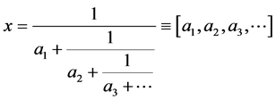 (2.1)
(2.1)
be the continued fraction expansion of the number . By applying Euclid’s algorithm one sees that the above expansion terminates if and only if x is a rational number. For x irrational one can construct recursively a sequence
  of rational approximants of x as
 (2.2)
(2.2)
We can write this recursion in matrix form as follows: letting
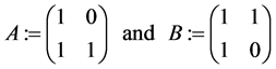 (2.3)
(2.3)
and noting that
 (2.4)
(2.4)
we have
 (2.5)
(2.5)
and
 (2.6)
(2.6)
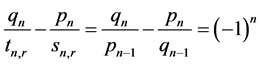
A short manipulation of (2.2) gives . Since
 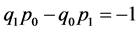 one obtains inductively the Lagrange formula
 (2.7)
(2.7)
Another useful formula which can be easily obtained from (2.2) is the following: for all  and
and ,
,
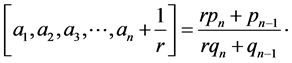 (2.8)
(2.8)
Letting  we get in particular
 (2.9)
(2.9)
Note that
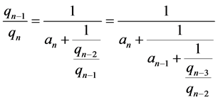
and so forth. We thus have the so called mirror formula (some consequences of which have been investigated in [4] ):
 (2.10)
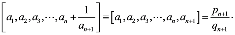
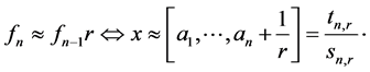
The numbers  are called continued fraction convergents (CFC) of x and it turns out that the n-th CFC
  is the best rational approximation to
  whose denominator does not exceed
  [2] . One sees that
 (2.11)
Putting  in (2.8) we get
 (2.12)
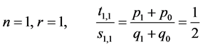
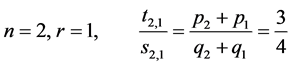
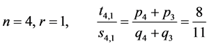
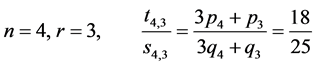
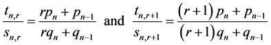
But what happens if  in (2.8) takes on an intermediate value
 ?
?
Definition 2.1 For  the sets
 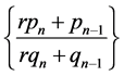 for
for  are the n’th Farey convergents (FC) for the real number
 .
.
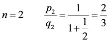
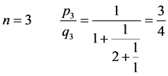
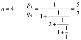
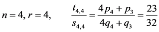
Example. Let . The first five CFC are


On the other hand, within the same accuracy, there are  FC’s. They are


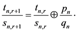
We now need some notions.
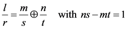
Definition 2.2 The Farey sum over two rationals  and
and  is the mediant operation given by
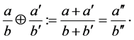 (2.13)
It is easy to see that  falls in the interval
  2. We say that
  and
and  are Farey neighbours if
 . Two Farey neighbours define a Farey interval and each Farey interval can be labeled uniquely according to the mediant (child)
  of the neighbours.
Observe that given a pair of consecutive FC’s, say
for some  and
and , we have
 (2.14)
Moreover
 (2.15)
by Lagrange’s formula. Therefore, for every , each FC
  for
for  is a Farey neighbour of
 , the corresponding Farey interval getting smaller and smaller as
  increases. More precisely, using again Lagrange’s formula, one easily obtains
 (2.16)
We therefore see that the FC  is the best one-sided rational approximation to
  whose denominator does not exceed
  (although, if
 , there might be a CFC with denominator less than
  and closer to
  on the other side of x). Increasing r, once we arrive at
  we hit a new CFC on the current side of
 , closer than the previous CFC. Finally, using matrix notation, the FC’s can be expressed in terms of intermediate products in (2.5) for
  as
as
 (2.17)
The algorithm which produces the sequence of  ‘s of a given real number is called slow continued fraction algorithm (see, e.g., [6] [7] ).
Remark 2.3 The set  of Farey fractions of order
  is the set of irreducible fractions in
  with denominator
![]() , listed in order of magnitude (see [8] ). Thus,
, listed in order of magnitude (see [8] ). Thus,  ,
,
and so on. In particular  with Euler totient function
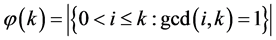 . Then we see that each
  for
for  is consecutive to
  in
in 
for .
.
2.1. Connection to Rotations of the Circle
One can interpret the above construction in terms of a kind of renormalization procedure for rotations of the circle  through an angle
 . With no loss we take the initial point to be the origin 0 and set
 .
.
Since  we have
  and thus
with
 (2.18)
Moreover we have

and therefore  or, which is the same,

with
 (2.19)
Iterating this procedure, we construct a family of nested intervals (see Figure 1) ,
,  , such that
 (2.20)
and
 (2.21)
where we have set . Using (2.18), (2.19) and (2.21) one gets inductively the formula
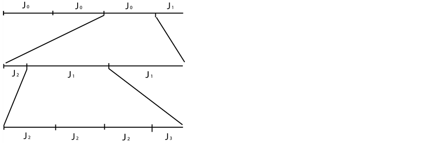
Figure 1. The construction of nested intervals.
 (2.22)
Note that
 (2.23)
Now, if we denote by  the euclidean metric on
  then
then
 (2.24)
Therefore
 (2.25)
That is, the sequence of arc-lengths  is but the sequence of successive closest distances to the initial point. This can be seen in the following way: starting from 0 and iterating
  times one ends up at the point
  which lies on the left of 0 and is the point closest to 0 up to now, being distant
 ![]() from it. Iterating
from it. Iterating  more times one ends up at the point
  which lies on the left of 0 at distance
 , ... iterating
  times one ends up at the point
  which still lies on the left of 0, at distance
 . One more iterate yields the point
  which now lies on the right of 0 at distance
  and is the point closest to 0 up to now, and so on and so forth (for more details see [9] ). The above implies that the first return map in the interval
  (which is
  or
or  according whether
  is even or odd) is the rotation through the angle
 . Finally, one has the equivalence:
 (2.26)
In addition, for each , it holds
 (2.27)
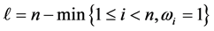
The three distance theorem. The points  with
with  partition the unit circle into
  intervals. A classical result (see e.g. [10] ), which can be easily obtained by induction using the above construction, is that the possible lengths of these intervals are organized according to the Farey convergents in the following way:
• If  then there are two distinct lengths:
  and
and  (which become
  and
and  when
when ).
).
• If 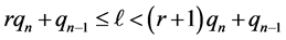 for some
  and
and  then there are at most three lengths:
 ,
,  and
and , the last of which disappears when
 .
.
We point out that in the second case above there are two intervals, chosen from among those having the smallest lengths:

which have 0 as their common endpoint. We then see that the approximations (26) and (27) are the same as shrinking one of these intervals to zero. Moreover, the fractions  and
and  are the two successive elements of
  having
  between them (see also Remark 2.3).
2.2. Growth of Denominators
The Gauss map  is defined as
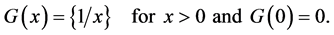 (2.28)
It is well known that  has an a.c. invariant ergodic probability measure
  given by
 (2.29)
A short reflection shows that  or else
 (2.30)
From this we obtain at once
 (2.31)
where the numbers  have been introduced in (2.22). Therefore
and, by the ergodic theorem, we have for  -almost all
  and then almost everywhere,
 (2.32)
Since  and thus
  another consequence of (2.30) is that

and therefore using (2.31)
 (2.33)
Putting together (2.32) and (2.33) we get the classical theorem of Lévy

On the other hand we may expect the growth of FC’s denominator to be subexponential. Indeed, let
 with
with  be the m-th FC. Its denominator satisfies
 . It is a result of Khinchin and Lévy (see [1] ) that

Combining the above we get the following
Lemma 2.4

Of course there are special behaviours: take , then
  and both are equal to the n-th Fibonacci number. Hence
  converge to
 .
.
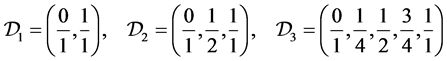
3. A Walk on the Farey Tree
Having fixed , let
, let  be the ascending sequence of irreducible fractions between 0 and 1 constructed inductively in the following way: set first
 , then
  is obtained from
  by inserting among each pair of neighbours
  and
and  in
in  their child
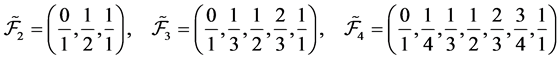
  as in (2.13). Thus

and so on. The elements of  are called again Farey fractions. Evidently
 .
.
Remark 3.1 It has been shown in ([11] , Thm 2.6) that the set  becomes equidistributed as
 . More specifically, the probability measure
  converges to the Lebesgue measure on
 .
.
Definition 3.2 For  we say that a Farey fraction
  has rank
  if
if .
.
We also define the . For
. For  there are exactly
  Farey fractions of rank
and their sum is equal to . Recall that every rational number
  has a unique finite continued fraction expansion
  with
with  [2] . The validity of the following relation will arise straightforwardly in the sequel:
Lemma 3.3

Remark 3.4 Note that, according to the above Lemma, the cardinality  of
of  can be interpreted as the number of choices of integers
 , with
  and so that
  for
for ,
, 
and . Indeed, for each fixed
  the number of such choices is
 , then sum over
 .
.
It is also easy to realize that all Farey fractions which fall in the interval  have rank greater than or equal to
 , whereas their continued fraction expansion starts with
 .
.
An interesting object is the Farey tree  whose vertex-set is
  and which is constructed as follows (see Figure 2):
• every column in  contains one entry (vertex or node);
• for  the
the  -th row is
 ;
;
• the node , representing the interval
 , is connected by edges to its left child
  and right child
  in the underlying row.

Figure 2. The first four levels of the Farey tree.
Note that the fractions  and
and  play the role of ancestors when using the Farey sum to obtain one row from the previous one. Besides the Farey sum, an alternative way to construct recursively the entries of
  is as follows.
Definition 3.5 Given  its descendants are the symmetrical entries of
  given by
  and
and respectively.
Lemma 3.6 The collection of all descendants of the entries of a given row in  is precisely the underlying row.
Proof. If  then
then  and
and . Therefore
 and the claim follows.
Remark 3.7 If  and
and  then
then  and
and .
.
3.1. The  Coding
Every rational number in  appears exactly once in the above construction and corresponds to a unique finite path on
  starting at the root node
  and whose number of vertices equals the rank of the rational number. We can code this path in the following way: first, any
  can be uniquely decomposed as3
 (3.1)
(3.1)
and the unimodular relations
 (3.2)
(3.2)
plainly hold. The neighbours  and
and  are thus the ‘parents’ of
  in
in  and we may accordingly identify
 (3.3)
(3.3)
with
 (3.4)
(3.4)
Note that the left column bears on the right parent and viceversa. Thus
 (3.5)
(3.5)
On the other hand, any  as above has a unique pair of (left and right) children, given by
 (3.6)
(3.6)
respectively. In order to generate them we set
 (3.7)
(3.7)
Note that for 
 (3.8)
(3.8)
and also
 (3.9)
(3.9)
Moreover, we have
 (3.10)
and
 (3.11)
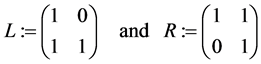
In other words, the matrices L and R, when acting from the right, move to the left and right child in , respectively. Moreover, it is plain that given
  we have
  and
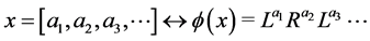
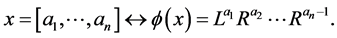
and . We have thus proved the following Proposition 3.8 To each entry
  there corresponds a unique element
  which, in turn, can be uniquely presented as
 (3.12)
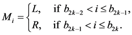
where the number of terms in the product  is equal to
  and Mi = L or Mi = R according whether the i-th turn, along the descending path in
  which starts from the root node
  and reaches xgoes left or right.
Remark 3.9 By the way, the matrices L and R induce the so called Farey tesselation of the upper half plane  (see [12] ).
Example.  is the right child of
 , which is the right child of
 , which is the left child of
 , which is the left child of
 . Thus

For , which is the left child of
 , we find

Note that .
.
To any given irrational number  we may associate a unique infinite path on
 , and thus a unique semi-infinite word in
 . Bearing in mind the continued fraction expansion (2.1) of x, let
the first FC of x. In order to reach it from the top of  we need the block
 . Whence we code x through the map
  defined by
 (3.13)
where  or
or  according whether the i-th turn along the infinite path in
  which starts from
 and approaches x along the sequence of successive FC’s goes left or right. This coding is faithful to the binary structure of
  but apparently not so much to the continued fraction expansion of x. To make the latter more transparent we may note that, according to the characterization of the FC’s given above (see (2.15) and (2.16)), the symbols L and R in (3.13) come in blocks whose lengths are given by nothing but the partial quotients
  of
of . More precisely, a short reflection shows that the following rule is in force: the first block is such that
  if
if . Moreover, for
  let
let

then we have
In other words, we have the coding
 (3.14)
Furthermore we set  and
and . More generally, we note that each rational x has two infinite paths which agree down to node
 : they are those starting with the finite sequence coding the path to reach x from the root node and terminating with either
  or
or . We shall agree that
  terminates with
  or
or  according whether the number of its (finite) partial quotients is even or odd. On the other hand, for notational simplicity’ sake we shall assume this agreement only implicitly. We summarize the above in the following Theorem 3.10 To
  with continued fraction expansion
  there corresponds a unique sequence
  given by
  which represents an infinite path on
  whose sequence of vertices starting from the
  -th is precisely the sequence
  of FC’s of x. Moreover, if
  denotes the lexicographic order on
  then
then
An simple consequence of the above construction is the following result.
Proposition 3.11 Let  with
with  and
and  even. Then its left and right children in
  are given by
  and
and , respectively. If instead
  is odd the expansions for
  and
and  have to be interchanged.
Proof. Since  is even we can write
 (3.15)
Therefore

which yield the claim. A similar reasoning applies for  odd.
odd. 
3.2. The {A, B} Coding
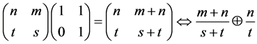
Using (3.9) we can write
 (3.16)
On the other hand we have  and (see (2.4))
 (3.17)
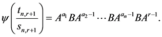
This defines a recoding  so that
 (3.18)
The FC  of
of , which has rank
 , will then be expressed as
 (3.19)
or else
 (3.20)
Note that both expansions have exactly  terms and the latter agrees with (2.17) once we interpret the l.h.s. of
(2.17) as the FC  of x, that is taking the Farey sum of the columns in the same spirit as (3.3).
Example. The example with 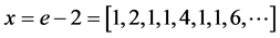 discussed above, which yields

can be used to check step by step what we are claiming here. For example its FC , which has rank 6, can be expressed as

3.3. The Farey Shift and Its Relatives
So far, a sequence in  starting with the symbol R has no image in
  with
with . Let us make the identification
 (3.21)
and denote by  the half-space of
  so obtained. We can write
 (3.22)
We see that the map  is a bijection between
  and
and .
.
Let  be the Farey shift map defined by
 (3.23)
Note that, besides  the only fixed point of
  is given by the sequence
  which is the image with
  of
of , the golden mean. This map acts on points in
  by reducing their rank of one unit.
For example, since , with the identifications made above we have


Let us define the Farey map  given by
 (3.24)
Its name can be related to the easily verified observation that the set of pre-images  coincides with
  for all
 . Note also that the
  -th row of the Farey tree is precisely
 . In particularthis implies that
 .
.
Proposition 3.12 Let  be the coding described above. Then

Proof. If  then
then  and
and . If instead
  then
then  and
and
 . Therefore,
 (3.25)
with . The claim now follows from (3.23) and (3.21).
3.3.1. The Gauss and Fibonacci Maps
The map F has (at least) two induced versions: the first one is the Gauss map 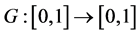 already introduced in (2.28), which for
  can be written as
 (3.26)
Recall that
 (3.27)
Noting that
 (3.28)
we see that G is obtained by iterating F once plus the number of times necessary to reach the interval . The second one is the Fibonacci map H and is defined by iterating F once plus the number of times necessary to reach the interval
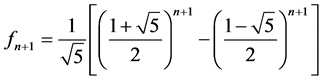
 . Let
. Let  and
and 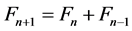 for
for  be the Fibonacci numbers. Then, for
 ,
,
 (3.29)
with
 (3.30)
In this case it is easy to check that if  then
then
 (3.31)
A sketch of the map F along its induced versions G and H is given in Figure 3.
Given  we may define the Möbius transformation
By the above, given  the point
  is but
  and for
  we have
 (recall that
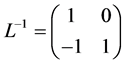 ). But what happens if
  so that
 ?
?
To see this we put
 (3.32)
We have

Therefore, noting that , for
, for  we have
 . To summarize we can represent the action of F as
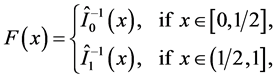
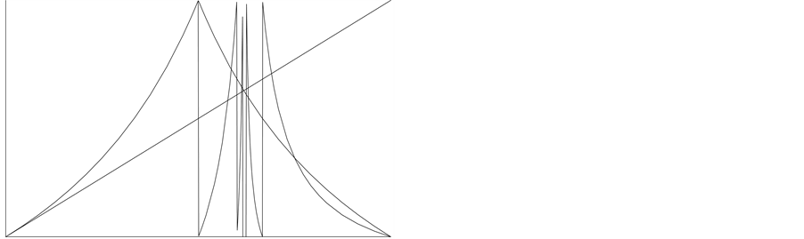

Figure 3. The Farey map and its induced Fibonacci (upper) and Gauss (lower) maps.
that of G as
and that of H as

3.3.2. The Modified Farey Map
Finally we introduce the modified Farey map  given by
 (3.33)
This map preserves orientation and has two indifferent fixed points, at 0 and 1. The advantage of using  instead of
  is that one can retrace the path from a leaf
  back to the root
 . More precisely, for
  let (cf. Proposition 3.8)
  be the element which uniquely represents x in
 . Then one easily sees that the following rule is in force: if
  then
then ,
,  then
then , for
, for  with
with  so that
 .
.
4. The Minkowski Question Mark
Given a number  with continued fraction expansion
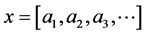 , one may ask what is the number obtained by interpreting the sequence
  (see (3.14)) as the binary expansion of a real number in
 . The number so obtained is denoted
  and writes
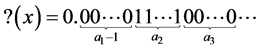 (4.1)
(4.1)
or, which is the same,
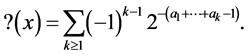 (4.2)
(4.2)
For instance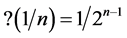 , for all
  (see Figure 4). Setting
  and
and  one has the following properties for the function
  (see [13] -[16] ):
•  is strictly increasing from 0 to 1 and Hölder continuous of exponent
 ;
;
• x is rational iff  is of the form
 , with k and s integers;
• x is a quadratic irrational iff  is a (non-dyadic) rational;
•  is a singular function: its derivative vanishes Lebesgue-almost everywhere.
The following additional properties easily follow from the definition.
Lemma 4.1  satisfies the functional equations


Proof. Assuming that  we write
  with
with  and
and . Setting moreover
  we have
  and
and . The assertion now follows by direct application of (4.2).
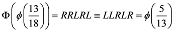
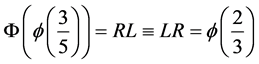
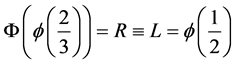
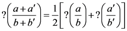
Let us now see how  acts on Farey fractions. We have already seen that
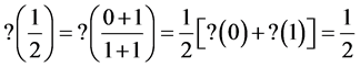
More generally, for any pair  and
and  of consecutive Farey fractions the function ? equates their child to the arithmetic average:
 (4.3)
(4.3)
One sees that the function ? maps the Farey tree  to the dyadic tree
  defined as follows: having fixed
 , let
, let  be the ascending sequence of fractions of the form
 ,
,![]() . We have
. We have
and so on. Then  is the same graph as
  with the
  -th row replaced by
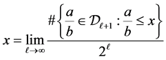
 . An immediate consequence of the fact that
  is that
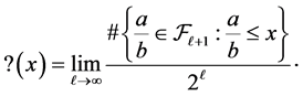
  is the asymptotic distribution function of the sequence of Farey fractions:
Theorem 4.2 Since
then
Remark 4.3 This result can be also deduced as a consequence of a more general result obtained in [17] using a suitable enumeration of the rationals in . As for the convergence of the atomic measure concentrated on
  to
to  see [11] and [18] .
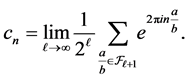
As a further immediate consequence we get that the Fourier-Stieltjes coefficients of  are as in the following

Figure 4. The Minkowski ? function.
Corollary 4.4 Let
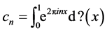
then
Finally, a short reflection using the definition (4.1) shows that ? conjugates the Farey map F and the modified Farey map  to the tent map
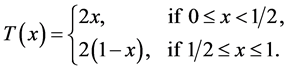 (4.4)
(4.4)
and the doubling map , respectively. Indeed, for any
  with
with  we have
 (4.5)
(4.5)
and
 (4.6)
(4.6)
where  and
and . A similar reasoning applies for D. Putting together the above, (3.25) and (4.1) we then get the following commutative diagrams
Theorem 4.5

This implies that the measure  is invariant under both maps F and
 , and its entropy is equal to
 . This makes
  the measure of maximal entropy for F and
 . Being zero at every rational point
  is of course singular w.r.t. Lebesgue. More specifically,
  is concentrated on a subset
  having Hausdorff dimension
  (see [14] ). In view of (3.25), the above has the following straightforward consequence Lemma 4.6 If x is drawn from
  according to the singular measure
 , then the partial quotients
  of
of 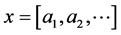 form a sequence of i.i.r.v.’s with
 .
.
It is moreover easy to realize that F and  have also absolutely continuous (not normalizable) invariant measures, with densities
 ![]() and
and , respectively.
Finally, the conjugacy of Theorem 4.5 has been used in [19] to construct a correspondence between the parameter spaces of  -continued fraction transformations and unimodal maps.
5. Transfer Operators and Partition Functions
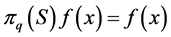
To a given matrix  and complex parameter
  one can associate the positive operator
 acting on the right as [20]
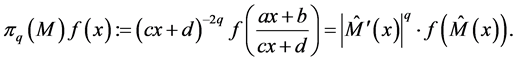 (5.1)
(5.1)
For example we have
 (5.2)
(5.2)
The operator  associated in this way to the map
  turns out to be the transfer operator acting as
 (5.3)
(5.3)
Of special significance is the (Perron-Frobenius) operator  which satisfies
 (5.4)
(5.4)
and has norm at most one in the Banach space . A function
  is the density of an absolutely continuous invariant measure for F if and only if
 . In this case we find
 , which however does not lie in
  (see [21] ).
Let f be an eigenfunction of  analytic in the half-plane
 . It satisfies
 (5.5)
(5.5)
and also
 (5.6)
(5.6)
Therefore the eigenvalue equation is equivalent to the three-term equation
 (5.7)
(5.7)
which is a generalisation of the Lewis functional equation (with ) studied in number theory (see [20] [22] ). The study of this generalized equation has been initiated in [23] .
Remark 5.1 In the context of the thermodynamic formalism, once a one-sided shift  and a potential function
  are given one defines a transfer operator
  on
on  by
by
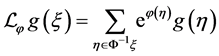
which plays a key role in the study of equilibrium states for  and their properties [24] [25] . In particular, one defines
and it turns out that if  decays exponentially then there is a unique mixing equilibrium state.
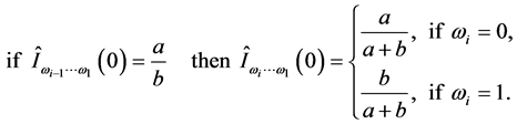
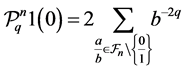
Relying on the above discussion it is now easy to see that  with
with

In order to compute  we have to consider points sharing the same path up to the k-th row of
 . Take for instance
  and
and . Then a short reflection yields, for
 ,
,
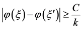
We therefore see that although  (so that
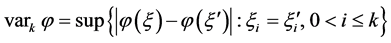
  is uniformly continuous)
  it is not even of summable variation. This entails that
  has indeed two equilibrium states, thus exhibiting a phase transition (see [26] ).
Next, we express the n-th iterate of  as
as
 (5.8)
(5.8)
where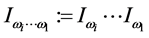 . We have
  so that, in particular, putting
  we get
 (5.9)
(5.9)
and
 (5.10)
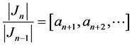
Lemma 5.2 Let  be the sequence of functions defined by
  and
and

For each fixed  we have that
  determines a bijection between
  and the set of denominators of the elements of
  (considered as an ordered set).
Proof. The proof is just a straightforward verification. Suppose for instance that  with
with
 , so that
 . Then by (5.9) and (5.10)
  is given by a product with
  factors of the type
  where r = a if
 , r = b otherwise. The result now readily follows by lemma 3.6.
Remark 5.3 The rank of the elements of  with denominator
  is given by
 with the convention
 . The smallest of the above denominators is 1, it has rank 0 and is obtained as
 . The two largest ones are equal to the
  -st Fibonacci number
 . They are symmetrical w.r.t
 , have rank
  and are obtained as
 and
and , respectively. More generally, it is not difficult to see that the following equivalence is in force: suppose that the element
  has rank
  so that
 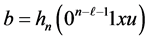 for some
  and
and , then the same denominator
 , but corresponding to the symmetrical fraction
 , is obtained as
  with
with .
.
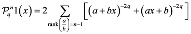
A direct consequence of the above lemma is the following
Theorem 5.4
Remarkably, the above sum is equal to the partition function  at (inverse) temperature
  of the number-theoretical spin chain introduced by Andreas Knauf in [27] . For
  we have (see [28] )
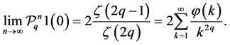 (5.11)
Note that for  the above limit diverges. This reflects the fact that the invariant density for the Farey map F, that is the fixed point of the operator
 , is the function
![]() .
.
Let us define the pressure function  as
as
 (5.12)
Since the sum in Thm. 5.4 has  terms we see that
  (this is the topological entropy of the map
 ). More generally let
  denote the sequence of denominators of the elements of
 when the latters are arranged in increasing order in
 , so that
 (5.13)
The ratio  can be interpreted as the moment of order
  of the size of the denominators in
 .
.  is plainly non-increasing and for
  satisfies
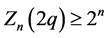 . Moreover we have
with ![]() for all
for all . Noting that
  we get for
Since  this yields
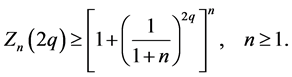 (5.14)
Thus, for all ,
,
 (5.15)
In addition, since  is non-increasing and
  (because the spectral radius of
  is 1, see above) we have
  for
for . Note that the same conclusion follows at once from the fact that
  is finite for
  (see (11)).
Remark 5.5 It holds 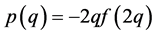 where
where  is the free energy of the Knauf model. In the context of thermodynamic formalism the pressure
  is a central object. In particular it is used as a generator of averages: its first derivative
 , wherever it exists, yields the mean of the function
  w.r.t. the equilibrium measure
![]() , which can be defined as the weak *-limit point of atomic measures supported on periodic points of F weighted with the function
, which can be defined as the weak *-limit point of atomic measures supported on periodic points of F weighted with the function  [24] . Note that
  for
for  and
and  as
as . On the other hand we have already seen that
 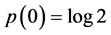 and
and  is called measure of maximal entropy. Higher derivatives of
  are connected to (sums of) higher correlation functions, see [25] [29] .
Let us now study the asymptotic behaviour of  for
for . To this end, we notice that if, instead of
 , we evaluate the iterate
  at
at , all sequences
  in (5.8) yield paths which end up at the same row of the Farey tree. The same argument leading to Theorem 5.4 now yields the following
Corollary 5.6
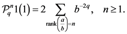 (5.16)
By Thm. 5.4 and (5.16) we obtain
 (5.17)
so that we can directly apply the results obtained by Thaler in [30] to get4
Lemma 5.7

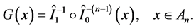
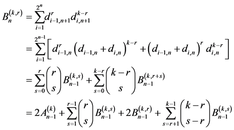
Lastly, noting that

one may then use , along with Lemma 3.6, to proceed inductively with
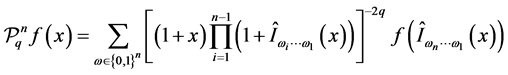
  in (5.8), and obtain the following general expression for
  with
with .
.
Theorem 5.8 For all  and
and  we have
We refer to [31] for further generalisations and applications (see also [32] ).
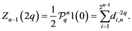
The Partition Function for Negative Integer Temperatures
Finally, we compute the value of the partition function  for some some specific value of the temperature. Related results are discussed in [33] (see also [34] ).
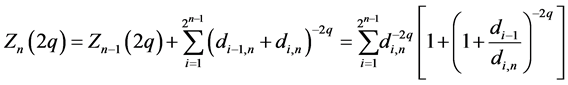
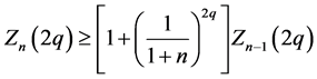
Lemma 5.9 We have, for all ,
,
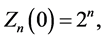
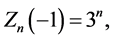
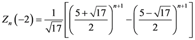
Proof. The first identity is trivial. The second one follows immediately from  along with (5.14), which gives the recursion
 . As for the third one, we can reason as follows: let us denote
 and
and . Then (5.14) yields
 . Moreover, we have

This yields the recursion  with
with  and
and  and the claim easily follows
 . The above result indicates a general argument to work out
  for any
 : setting
  and
and  one has

and
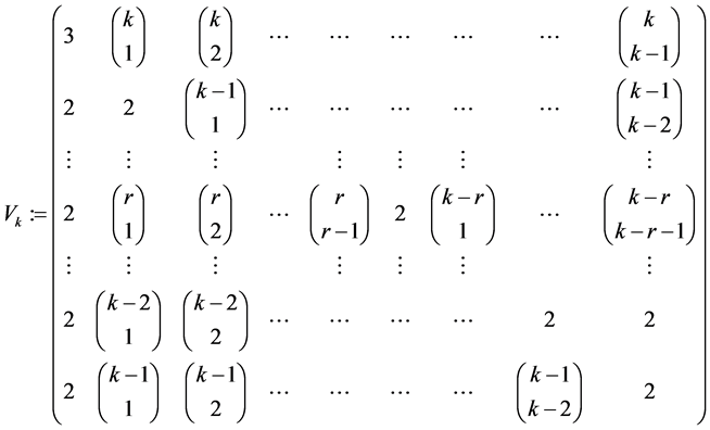
This yields a k-dimensional recursion
 (5.18)
with  matrix
and initial condition
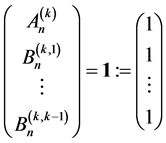 (5.19)
By Perron-Frobenius theorem the matrix  has a simple real positive maximal eigenvalue
  whose eigenvector
  has strictly positive components. This immediately yields
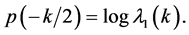 (5.20)
More specifically, by the above the exact behaviour of  can be obtained by standard linear algebra. If for instance
  can be diagonalized with spectrum
 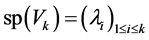 and corresponding eigenvectors
 , then we can expand
  so that (5.18) and (5.19) yield
 (5.21)
where  denotes the first component of
 . On the other hand, as we shall see in the forthcoming example,
  is not always diagonalizable.
Examples. For  we find

so that by (5.20)  and using (5.21) one easily recover the result of Lemma 5.9 for
 .
.
For  we get
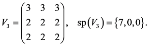
In this case (5.21) does not hold but one easily finds
and .
.
The case  is still different, yielding

References
- Khinchin, A.Y. (1964) Continued Fractions. The University of Chicago Press, Chicago.
- Hardy, G. H. and Wright, E. M. (1979) An Introduction to the Theory of Numbers. Oxford University Press, Oxford.
- Hensley, D. (2006) Continued Fractions. World Scientific, Singapore City.
- Adamczewski, B. and Allouche, J.P. (2007) Reversal and Palindromes in Continued Fractions. Theoretical Computer Science, 380, 220-237. http://dx.doi.org/10.1016/j.tcs.2007.03.017
- Farey, J. (1816) On a Curious Property of Vulgar Fractions. London and Edinburgh Philosophical Magazine and Journal of Science, 47, 385-386.
- Appelgate, H. and Onishi, H. (1983) The Slow Continued Fraction Algorithm via 2 × 2 Integer Matrices. The American Mathematical Monthly, 90, 443-455. http://dx.doi.org/10.2307/2975721
- Lagarias, J.C. (2001) The Farey Shift and the Minkowski ?-Function. Preprint.
- Apostol, T. (1976) Modular Functions and Dirichlet Series in Number Theory. Graduate Texts in Mathematic 41, Springer, New York. http://dx.doi.org/10.1007/978-1-4684-9910-0
- Bonanno, C. and Isola, S. (2009) A Renormalization Approach to Irrational Rotations. Annali di Matematica Pura ed Applicata, 188, 247-267. http://dx.doi.org/10.1007/s10231-008-0074-5
- Alessandri, P. and Berthè, V. (1998) Three Distances Theorem and Combinatorics on Words. L’Enseignement Mathématique, 44, 103-132.
- Conze, J.P. and Guivarc’h, Y. (2002) Densité d’orbites d’actions de groupes linéaires et propriétés d’équidistribution de marches aléatoires. In: Burger, M. and Iozzi, A., Eds., Rigidity in Dynamics and Geometry (Cambridge 2000), Springer, Berlin, 39-76.
- Knauf, A. (1999) Number Theory, Dynamical Systems and Statistical Mechanics. Reviews in Mathematical Physics, 11, 1027-1060. http://dx.doi.org/10.1142/S0129055X99000325
- Salem, R. (1943) On Some Singular Monotone Functions Which Are Strictly Increasing. Transactions of the American Mathematical Society, 53, 427-439. http://dx.doi.org/10.1090/S0002-9947-1943-0007929-6
- Kinney, J.R. (1960) A Note on a Singular Function of Minkowski. Proceedings of the American Mathematical Society, 11, 788-794.
- Bonanno, C. and Isola, S. (2009) Orderings of the Rationals and Dynamical Systems. Colloquium Mathematicum, 116, 165-189. http://dx.doi.org/10.4064/cm116-2-3
- Alkauskas, G. (2010) The Minkowski Question Mark Function: Explicit Series for the Dyadic Period Function and Moments. Mathematics and Computation, 79, 383-418. http://dx.doi.org/10.1090/S0025-5718-09-02263-7
- Viader, P., Paradis, J. and Bibiloni, L. (2001) A New Light on Minkowski’s ?(x) function. Journal of Number Theory, 73, 212-227. http://dx.doi.org/10.1006/jnth.1998.2294
- Gouëzel, S. (2009) Local Limit Theorem for Non-Uniformly Partially Hyperbolic Skew-Products and Farey Sequences. Duke Mathematical Journal, 147, 192-284. http://dx.doi.org/10.1215/00127094-2009-011
- Bonanno, C., Carminati, C., Isola, S. and Tiozzo, G. (2013) Dynamics of Continued Fractions and Kneading Sequences of Unimodal Maps. Discrete and Continuous Dynamical Systems, 33, 1313-1332. http://dx.doi.org/10.3934/dcds.2013.33.1313
- Lewis, J.B. and Zagier, D. (1997) Period Functions and the Selberg Zeta Function for the Modular Group. In: Drouffe, D.M. and Zuber, J.B., Eds., The Mathematical Beauty of Physics, Advanced Series in Mathematical Physics, Vol. 24, World Scientific, River Edge, 83-97.
- Isola, S. (2002) On the Spectrum of Farey and Gauss Maps. Nonlinearity, 15, 1521-1539. http://dx.doi.org/10.1088/0951-7715/15/5/310
- Lewis, J.B. (1997) Spaces of Holomorphic Functions Equivalent to Even Maass Cusp forms. Inventiones Mathematicae, 127, 271-306. http://dx.doi.org/10.1007/s002220050120
- Bonanno, C. and Isola, S. (2014) A Thermodynamic Approach to Two-Variable Ruelle and Selberg Zeta Functions via the Farey Map. Nonlinearity, to appear.
- Bowen, R. (1976) Equilibrium States and Ergodic Theory of Anosov Diffeomorphisms. Lecture Notes in Mathematics, 470.
- Ruelle, D. (1978) Thermodynamic Formalism. Addison-Wesley Publishing Company, Boston.
- Isola, S. (2003) On Systems with Finite Ergodic Degree. Far East Journal of Dynamical Systems, 5, 1-62.
- Knauf, A. (1998) The Number-Theoretical Spin Chain and the Riemann Zeros. Communications in Mathematical Physics, 196, 703-731. http://dx.doi.org/10.1007/s002200050441
- Knauf, A. (1993) On a Ferromagnetic Spin Chain. Communications in Mathematical Physics, 153, 77-115. http://dx.doi.org/10.1007/BF02099041
- Kotani, M. and Sunada, T. (2001) The Pressure and Higher Correlations for an ANOSOV Diffeomorphism. Ergodic Theory and Dynamical Systems, 21, 807-821. http://dx.doi.org/10.1017/S0143385701001407
- Thaler, M. (1995) A Limit Theorem for the Perron-Frobenius Operator of Transformations on [0,1] with Indifferent Fixed Points. Israel Journal of Mathematics, 91, 111-127. http://dx.doi.org/10.1007/BF02761642
- Degli Esposti, M., Isola, S. and Knauf, A. (2007) Generalized Farey Trees, Transfer Operators and Phase Transitions. Communications in Mathematical Physics, 275, 297-329. http://dx.doi.org/10.1007/s00220-007-0294-3
- Boca, F. (2007) Products of Matrices
 and
and  and the Distribution of Reduced Quadratic Irrationals. Journal für die reine und angewandte Mathematik, 2007, 149-165.
 - Bonanno, C., Graffi, S. and Isola, S. (2008) Spectral Analysis of Transfer Operators Associated to Farey Fractions. Rendiconti Lincei-Matematica e Applicazioni, 19, 1-23. http://dx.doi.org/10.4171/RLM/505
NOTES

1Good general sources on this subject are -.

2The origin of these names traces back to Cauchy, who proved this property after it was observed by John Farey in 1816 , and named “Farey series” the numbers obtained in this way.

3All fractions are supposed in lowest terms.

4We say that an and bn are asymptotically equivalent, denoted as an ~ bn, if the quotient an/bn tends to unity as n approaches ∞.