Applied Mathematics
Vol.4 No.4(2013), Article ID:30367,10 pages DOI:10.4236/am.2013.44085
Some One Parameter Models for Continuous Random Variables Defined on the Interval [0, 1]
The University of Texas at Dallas, Richardson, USA
Email: wiorkow@utdallas.edu
Copyright © 2013 John J. Wiorkowski. This is an open access article distributed under the Creative Commons Attribution License, which permits unrestricted use, distribution, and reproduction in any medium, provided the original work is properly cited.
Received January 9, 2013; revised February 14, 2013; accepted February 21, 2013
Keywords: Probability Distribution; Risk Assessment; Reliability Assessment; PERT CPM
ABSTRACT
The Beta Distribution is almost exclusively used for situations, after range normalization, wherein a continuous random variable is defined on the closed range [0, 1]. Since the beta distribution is intrinsically a two parameter distribution, this creates problems in some applications where specification of more than one parameter is difficult. In this note, two new classes of single parameter continuous probability distributions on a closed interval are introduced. These distributions remove some of the theoretical and practical problems of using the Beta Distribution for applications. The Burr Type XI Distribution has desirable characteristics for many applications especially when there is ambiguity in the definition of the specified parameter.
1. Introduction
The standard two parameter Beta Distribution is the most widely used distribution for situations wherein a continuous random variable is confined to a bounded interval . After appropriate normalization to the interval
 , the Beta Distribution provides a flexible family of probability density functions capable of modeling a wide variety of natural phenomena. There are situations, however, where the Beta Distribution cannot model natural phenomena or its use is problematic. In their recent book, Kotz and van Dorp [1] introduce and discuss the properties of other continuous families of distributions with bounded support. This widely extends the types of natural phenomena which can be modeled. But even this wide array of probability distributions have problems when modeling a low risk event. Consider the problem of providing a distribution for the situation where a subject matter expert subjectively estimates that the probability of a risky event as 0.01. Since the Beta Distribution is a two parameter model, this single estimate is inadequate for determining an appropriate Beta Distribution model. Except for the Triangular Distribution, all the alternative models in Kotz and van Dorp [1] are also at least two parameter models and thus indeterminate based on a single estimate of the risk probability. A substantial literature exists to aid the statistician in eliciting further information from subject matter experts to remove this indeterminacy (see O’Hagan et al. [2] for a review of the area). These techniques involve specifying a numerical estimate for another characteristic of the distribution such as the mean or a percentile. Taking the initial estimate as the mode and the estimate of some other distribution characteristic, allows a two parameter model to be fit (See Donaldson [3], Johnson [4], Lau, A. et al. [5], Lau H. et al. [6], Mohan et al. [7] and Premachandra [8]. Another example involves the management of large scale complex projects. A common methodology used in this situation is called PERT-CPM (Program and Evaluation and Review Technique-Critical Path Method). This technique has been used for the development of the Polaris Missile System and also for planning and managing the hosting activities of the International Olympics. In this approach the large project is broken down into a myriad of component parallel or sequential activities, each of which are uncertain in duration. Experts are asked to provide estimates of durations of these components. But as stated by Fazar [9] “PERT quantifies knowledge about the uncertainties involved in developmental programs requiring effort at the edge of, or beyond, current knowledge of the subject—effort for which little or no previous experience exists”. In discussion with individuals involved in either of these two situations, I have found that although they are comfortable in providing a subjective “most likely” estimate of an event, most would have difficulty specifying any other characteristic of the distribution. Indeed many seem to hold that their subjective estimate is not only the most likely, (corresponding to the mode of the distribution) but simultaneously would be willing to give even odds that the actual probability is above or below their estimate (corresponding to the median). This ambiguity has also been reported by Trout [10]. Accordingly, there is a need for one parameter probability models to handle the real situation of having only one reliable estimate from a subject matter expert and for which the mode and median are very close. Of course it is possible to create probability distributions where the mode and median exactly coincide, however, there may be circumstances where other criteria may be paramount so that general methods for creating one parameter distributions may be of value.
2. Tilted Distributions
Exponential tilting is a well known method (See Davison [11] Section 5.2 for example) which can be used to induce a one parameter family of distributions. Let  denote a probability density function on the closed interval
  with the property that
  and such that,
 (1).
(1).
Define the moment generation function of  as,
as,
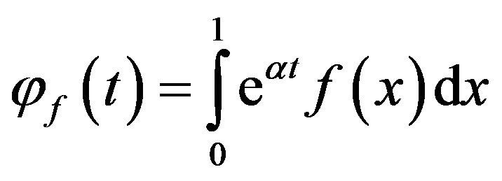 (2)
(2)
then
 (3)
(3)
is also a probability density function on the closed interval . If
. If  has no parameters, then
  defines a one parameter family on
  with parameter t, where t can range over the interval
 ![]() to
to![]() . The probability density function
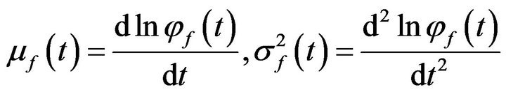
. The probability density function  has several desirable properties. First, the moment generating function of
  is given by
  so that the mean and variance of the density function are given by the equations
 (4)
(4)
from which explicit formulae for the mean and variance can be obtained. The function  is the cumulant generating function of the density
 . Secondly, the form of (3) implies that
  is in the exponential family of distributions. This family of distributions has been well studied and has several desirable properties. For example, in this case, if one has a random sample from
 , then one can obtain the maximum likelihood estimate of t by simply setting the sample mean equal to
  and solving for t. The asymptotic variance of this estimate if given by
 . Finally, if
 is a concave function, then t can be uniquely related to the mode,
 ![]() , through the relationship,
, through the relationship,
 (5)
(5)
where  is the first derivative of
  with respect to x, evaluated at
![]() . This means that one can specify a distribution by specifying the mode
. This means that one can specify a distribution by specifying the mode![]() , use (5) to find t, and then use (4) to determine the basic statistical properties of the distribution.
, use (5) to find t, and then use (4) to determine the basic statistical properties of the distribution.
The choice of  is extremely broad, but as pointed out by one of the referees, it is best to start with
  which is symmetric about the point
  to guarantee that any modal value between 0 and 1 can be modeled As examples of the above, consider three simple choices for
  on the closed interval
 . The first is the Beta (2, 2) distribution with probability density function,
 (6)
(6)
The second is the Gilbert distribution (Edwards [12]) with probability density function,
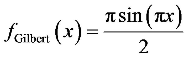 (7)
(7)
The third is a translated version of the Raised Cosine distribution (Proakis [13], p. 189), and is also a special case of the Burr Type XI distribution (Burr [14] and Kotz and Johnson [15], p. 335). It has probability density function,
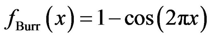 (8)
(8)
These probability density functions are shown in Figure 1. As can be seen, the Beta (2, 2) and Gilbert densities are quite close to one another. Further, the Burr density differs distinctly from the other two being much more concentrated around the value 0.5, and showing much greater tapering as x approaches 0 or 1. (As pointed out by the referee, in some applications one might prefer to start with symmetric beta distributions but the above three choices illustrate the distribution construction approach adequately.)
Figure 2 shows the three tilted distributions with a mode, ![]() , of 0.01. The values of t corresponding to a mode of 0.01 are –98.9898 for the tilted beta, –99.9671 for the tilted Gilbert, and –199.9342 for the tilted Burr distribution.
, of 0.01. The values of t corresponding to a mode of 0.01 are –98.9898 for the tilted beta, –99.9671 for the tilted Gilbert, and –199.9342 for the tilted Burr distribution.
As can seen, the tilted Beta and Gilbert densities are
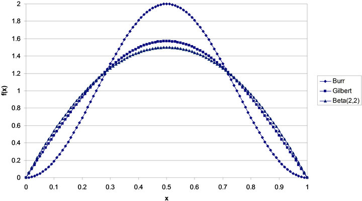
Figure 1. Probability density functions.
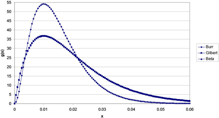
Figure 2. Tilted density functions mode = 0.01.
almost indistinguishable and quite distinct from the tilted Burr density. This similarity between the tilted Gilbert and tilted Beta distributions seems to be typical for both low and high values of the mode![]() .
.
The skewness of the distributions might be viewed as a desirable characteristic if one believed that experts tend to underestimate the probability of rare events. (In a reliability situation with a mode say of 0.99, the tilted densities would be left skewed and model a situation wherein experts tend to overestimate the reliability.)
Figure 3 shows the relationship between ![]() and
and  for the three tilted distributions. The closer
  is to 0.5, the closer the median and mode of the distributions are (Berny [16] uses one minus this probability as a parameter in his model).
Again, there is almost no difference between the tilted Beta and tilted Gilbert distributions over the whole range of the mode![]() . Further the probabilities of being less than the mode for the tilted Burr distribution are uniformly closer to 0.5 than the other two distributions. However, the deviation from 0.5 is large even for the tilted Burr distribution. Accordingly, if one agreed with Trout [10], none of these distributions would provide Adequate models for modeling expert assessment of
. Further the probabilities of being less than the mode for the tilted Burr distribution are uniformly closer to 0.5 than the other two distributions. However, the deviation from 0.5 is large even for the tilted Burr distribution. Accordingly, if one agreed with Trout [10], none of these distributions would provide Adequate models for modeling expert assessment of
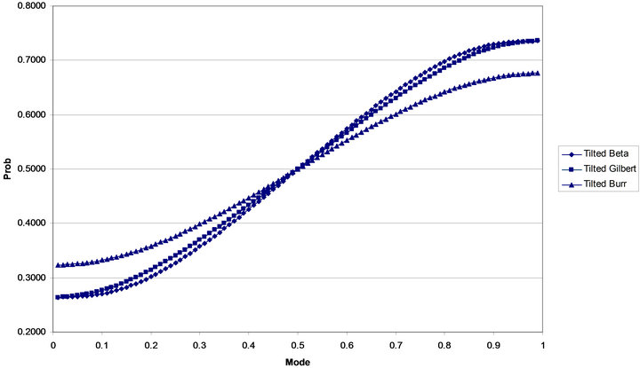
Figure 3. Probability of being less than the mode.
probabilities since the modes and medians do not seem close.
3. MAX Distributions
Let  be the cumulative probability distribution function corresponding to the probability density function
  on
on , i.e.
 (9)
(9)
Then for ,
,  is also a cumulative probability distribution function on the range
 . Indeed, if K is an integer, n, then
  is the cumulative distribution function of the maximum value of X from a random sample of size n where X has probability density function
 . Define,
 (10)
(10)
then  is a probability density function on
 . Further,
  is also a probability density function, the rotated image of
  about the fixed point
 . If
. If  and
and  are both concave, then
  has a unique mode
 ![]() on
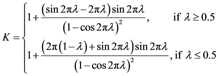
on . Under these conditions, it is straightforward to show that the relationship between K and
 ![]() is given the by the equations,
is given the by the equations,
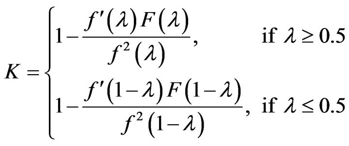 (11)
(11)
where  is the first derivative of
  with respect to x. Accordingly, one can generate a probability distribution by specifying the mode
![]() , use (11) to find K and if the mode is greater than 0.5 use (10) to find the density function. If the mode is less than 0.5, then one uses (10) with x replaced by
, use (11) to find K and if the mode is greater than 0.5 use (10) to find the density function. If the mode is less than 0.5, then one uses (10) with x replaced by . Percentiles xp for the density
  can easily be found by solving the equation
 (12)
(12)
Unfortunately, the form of (10) does not lend itself to closed form solutions for moments.
If one has a random sample of size n from , then the maximum likelihood of K is,
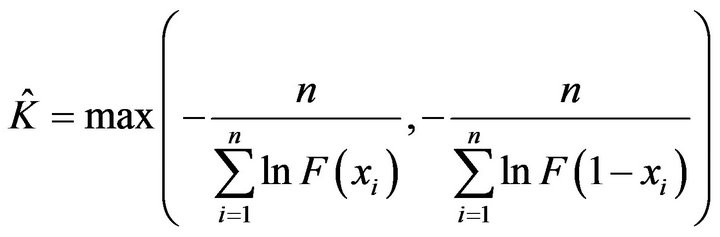 (13)
(13)
with asymptotic variance . A form of this distribution was discussed by Topp and Leone [17] and further discussed in Kotz and van Dorp [1].
Figure 4 shows the three MAX distributions for the case . The BetaMAX distribution would have K = 1667, the GilbertMAX distribution would have K = 2026.59, and the BurrMAX distribution would have K = 101321.5.
As can be seen, as in the case of the Tilted distributions, the BetaMAX and GilbertMAX densities are indistinguishable and quite distinct from the BurrMAX distribution. Both the BetaMAX and GilbertMAX distributions show right skew (they would be left skewed if ) while the BurrMAX is almost symmetric. In contrast to the Tilted distributions shown in Figure 2, the Max distributions are much less variable with almost all the probability mass confined to the range 0 to 0.03. This is a much smaller range than the Tilted Beta and Tilted Gilbert which essentially go from 0 to 0.06. Accordingly, if one expected greater underestimation of probabilities by experts, the Tilted distributions would be preferred. However, as mentioned earlier, it may be the case that when asked to determine “most likely” values, experts are estimating the median rather than the mode.
Accordingly, in Figure 5, the probability of being less than the median is plotted as a function of the mode for the three Max densities discussed in this paper.
Figure 5 is plotted on the same scale as Figure 3. It is immediately clear, that all of the Max distributions have modes which are much closer to the median. The median and mode are remarkably close for the BurrMAX distribution, with  differing from 0.5 by a maximum value of 0.0281 at approximately λ = 0.28 and 0.72. Accordingly, the Max distributions seem better suited for handling the ambiguity of expert estimation of the “most likely value”. Specifically, the BurrMax distribution, for which the mode and median are extremely close over whole range of possible values, seems an useful one parameter distribution for applications wherein individuals are asked to provide “most likely values”.
4. The BurrMAX or Burr Type XI Distribution
When ![]() is the Burr distribution, (11) can be written as
is the Burr distribution, (11) can be written as
 (14)
(14)
With the appropriate value of K, the cumulative distribution function of the Burr Type XI distribution is given by
 (15)
(15)
The first equation in (15) was first given by Burr [14], and given the designation Type XI by Kotz and Johnson [15] Vol. 1, p. 335, in their discussion of the Burr Family of distributions. The probability density functions of the BurrMAX distributions are
 (16)
(16)
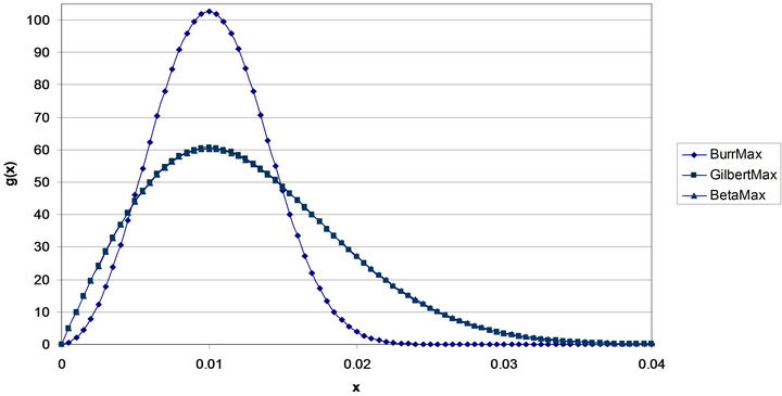
Figure 4. Max density functions mode = 0.01.
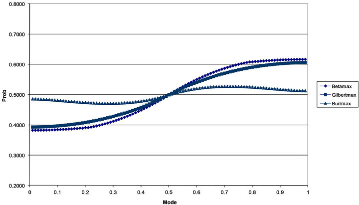
Figure 5. Probability of being less than the mode.
Since (14) are mixed trigonometric equations, there is no closed form equation to find the mode, ![]() , given K .
, given K .
The median,  , or indeed any percentile xp, for
 , can be obtained by solving the equation
 (17)
(17)
which, since it is a mixed trigonometric equation, has no closed form solution. Equation (17), however, can be solved using numerical procedures. If , then to find xp, replace p with
  in (54), solve, and subtract the solution from 1.
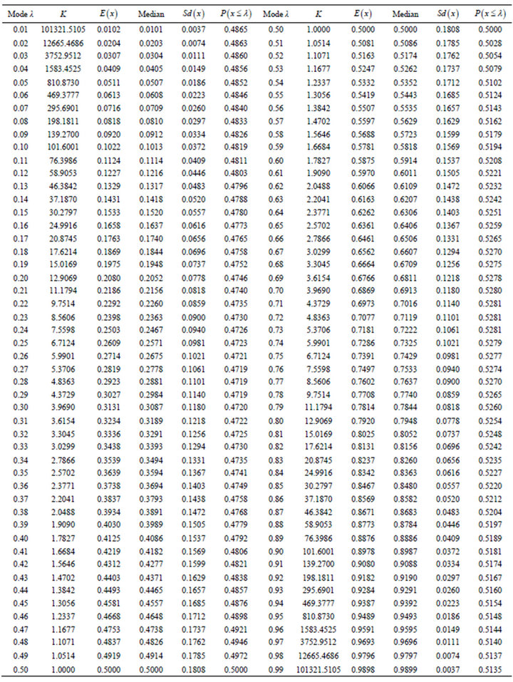
No closed form solution or general numerical solutions can be found for the mean and standard deviation of the Burr Type XI distribution. Accordingly, direct numerical integration of the integrals defining the first and second central moments was performed to obtain the resulting means and standard deviations as given in Table 1.
5. Extreme Value Distribution Approximation
In risk situations where one estimates very small probabilities, or in a reliability context when one estimates probabilities very close to 1, use of a Max distribution becomes problematic as the values of K become very large. One can capitalize, however, on the fact that for K = n, an integer, all of the Max distributions can be thought of as representing the distributions of the maximum (if ) or the minimum (if
 ) of n random samples taken from the appropriate distribution. Accordingly, one can use the theory of extreme values and extend the results from integer values, n, to a continuous value
 .
.
Following the discussion in Johnson et al. [18] Chapter 22, the distribution of the maximum of a sample of size n, for large enough n, for the distributions discussed in this paper, converge in law to a Weibull distribution which for  has the cumulative distribution function is given by the equation
 (18)
(18)
If the value of ![]() can be determined, then the above distribution becomes a function of
can be determined, then the above distribution becomes a function of ![]() alone and is a one parameter distribution. In Johnson et al. [18] Chapter 22, a method is given for finding
alone and is a one parameter distribution. In Johnson et al. [18] Chapter 22, a method is given for finding ![]() based on the cumulative distribution function
based on the cumulative distribution function  of the initial generating distribution. The result is that
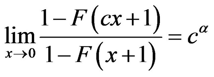 (19)
(19)
For the Burr distribution, (19) yields the value  so that for
  or
or  the theory of Extreme Value Distributions indicates that the Burr Type
Table 1. Characteristics of the Burr Type XI Distribution.
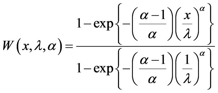
XI distribution can be closely approximated to nine decimal places by a Weibull extreme value distribution on the range . Specifically, the cumulative distribution function is given by
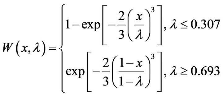 (20)
(20)
with corresponding probability density functions,
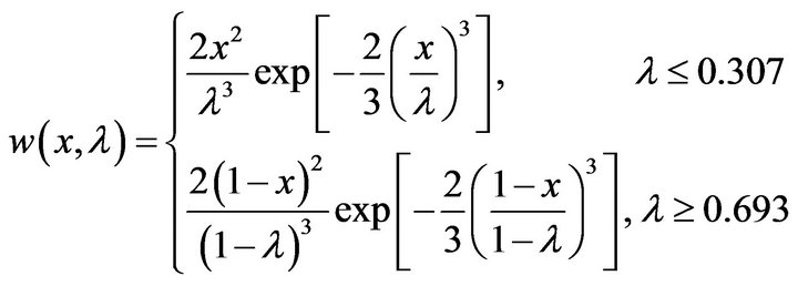 (21)
(21)
If , we have from the properties of the Weibull distribution [Johnson et al. [19] Chapter 21], that
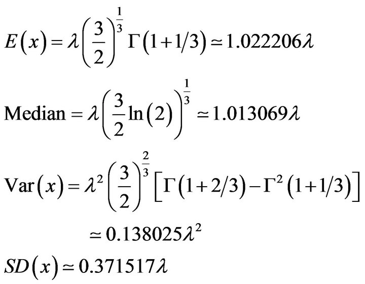 (22)
(22)
For , the corresponding results are,
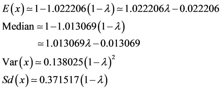 (23)
(23)
For the BetaMAX and GilbetMAX distributions, (19) indicates that  so that for λ ≤ 0.1473 or λ ≥ 0.8527 both distributions can be closely approximated to nine decimal places by a Weibull extreme value distribution on the range
  which coincides with a form of the Rayleigh distribution Johnson et al. (1995), Chapter 18, Section [10].
Figure 6 shows the Extreme value distributions for . As expected it’s appearance is similar to that of Figure 4. The distribution for
  (limiting value of the Burr Type XI distribution) has expected value of 0.0102, a median of 0.0101, and a standard deviation of 0.0037. When
  (limiting form of the GilbertMax and BetaMax distributions) the corresponding values are 0.0125, 0.0118, and 0.0066.
6. Applications
It is clear from the previous discussion that the Gilbert distribution and Beta (2, 2) distributions yield Tilted, MAX and Extreme Value distributions which are essentially numerically indistinguishable. Accordingly, I see no applications for any form of the Gilbert distribution. In risk or reliability studies, where ![]() would be expected to be close to 0 or close to 1 respectively, the Extreme value distributions would seem to be most useful. They have a relatively simple form and one can obtain good approximations to their moments using (20) and (21). Further one can obtain percentiles of the extreme value distributions using the formulas,
would be expected to be close to 0 or close to 1 respectively, the Extreme value distributions would seem to be most useful. They have a relatively simple form and one can obtain good approximations to their moments using (20) and (21). Further one can obtain percentiles of the extreme value distributions using the formulas,
 (24)
(24)
By replacing p or 1 − p in (24) with a uniformly distributed random variable U, one can easily simulate samples of any size from these distributions. The choice of whether to use  hinges on whether one believes that experts are truly estimating the mode and not the median. If they are, then choosing
  would seem to be preferred since it allows for expert under estimation of probabilities in the case of risk applications, or over estimation of probabilities in reliability applications. On the other hand, if there is ambiguity as to whether experts are estimating the mode or median when asked for the “most likely value”, then using the Extreme Value distribution with
  would seem most appropriate since for this distribution the median and mode are almost identical.
In PERT or stochastic CPM applications where ![]() would not be expected to be either very small or very large, the Extreme Value distributions would not be appropriate. Typically either the Triangle distribution with mode
would not be expected to be either very small or very large, the Extreme Value distributions would not be appropriate. Typically either the Triangle distribution with mode ![]() or the Beta distribution with mean
or the Beta distribution with mean  and standard deviation of
  have been used in this situation. The standard deviations of these two distributions as well as the BetaMax and Burr Type XI distributions are shown in Figure 7. Unlike the usual Beta approximation or Triangular distribution cases, the two Max distributions show the variability declining as the mode approaches 0 or 1.
It seems clear that the BetaMax and Burr Type XI distributions are better than both the usual Beta approximation model and Triangular distribution since for these
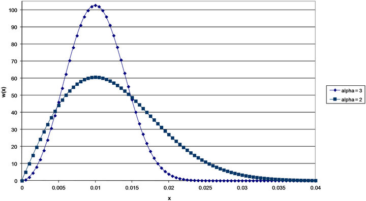
Figure 6. Weibull extreme value distributions mode = 0.01.

Figure 7. Standard deviations.
two distributions the variability is substantially lower as one moves away from the middle of the modal range. If one was worried about the ambiguity of the term “most likely value”, then one would use the Burr Type XI distribution instead of the Usual PERT model based on Figure 5 which shows the closeness of the median and mode of the Burr Type XI distribution. If this was not a concern then the choice would depend on one’s conception of variability. However, if one wanted to keep variability at a reasonable level, again one is led to the Burr Type XI distribution with a standard deviation which is between 0.36 and 0.39 the value of the mode (when the mode is below 0.5).
Perhaps the most useful application of these one parameter distributions is to allow experts with limited backgrounds in probability to more accurately specify their uncertainties about the situations they are working with. For example consider the problem of estimating the chances of a failure in a power system. The expert needs only to come up with one estimate, say 0.001, and the distributions discussed in this paper would automatically generate a plausible distribution for the uncertainty in this figure. Given that many risk assessment studies and complicated projects consist of hundreds to thousands of uncertain steps, the reduction in difficulty by using one parameter families should greatly ease the problem of assigning reasonable uncertainty to the myriad steps.
REFERENCES
- S. Kotz and J. R. van Dorp, “Beyond Beta, Other Continuous Families of Distributions with Bounded Support and Applications,” World Scientific Publishing Co., Singapore City, 2004.
- A. O’Hagan, C. Buck, A. Daneshkhah, J. Eiser, P. Garthwaite, D. Jenkinson, J. Oakley and T. Rakow, “Uncertain Judgements, Eliciting Experts’ Probabilities,” John Wiley and Sons, Ltd., Chichester, 2006. doi:10.1002/0470033312
- W. Donaldson, “The Estimation of the Mean and Variance of a PERT Activity Time,” Operations Research, Vol. 13, No. 3, 1965, pp. 382-385. doi:10.1287/opre.13.3.382
- D. Johnson, “The Triangular Distribution as a Proxy for the Beta Distribution in Risk Analysis,” The Statistician, Vol. 46, No. 3, 1997, pp. 387-398. doi:10.1111/1467-9884.00091
- A. Lau, H. Lau and Y. Zhang, “A Simple and Logical Alternative for Making PERT Time Estimates,” IIE Transactions, Vol. 28, No. 3, 1996, pp. 183-192. doi:10.1080/07408179608966265
- H. Lau, A. Lau and C. Ho, “Improved Moment-Estimation Formulas Using More than Three Subjective Fractiles,” Management Science, Vol. 44, No. 3, 1998, pp. 346-351. doi:10.1287/mnsc.44.3.346
- S. Mohan, M. Gopalakrishnan, H. Balasubramanian and A. Chandrashekar, “A Lognormal Approximation of Activity Duration in PERT Using Two Time Estimates,” Journal of the Operational Research Society, Vol. 58, No. 6, 2007, pp. 827-831. doi:10.1057/palgrave.jors.2602204
- I. J. Premachandra, “An Approximation of the Activity Duration Distribution in PERT,” Computers and Operations Research, Vol. 28, No. 5, 2001, pp. 443-452. doi:10.1016/S0305-0548(99)00129-X
- W. Fazar, “Program Evaluation and Review Technique,” The American Statistician, Vol. 13, No. 1, 1959, p. 10.
- M. Trout, “On the Generality of the PERT Average Time Formula,” Decisions Sciences, Vol. 20, No. 2, 1989, pp. 410-412. doi:10.1111/j.1540-5915.1989.tb01888.x
- A. Davison, “Statistical Models,” Cambridge University Press, London, 2003. doi:10.1017/CBO9780511815850
- A. Edwards, “Gilbert’s Sine Distribution,” Teaching Statistics, Vol. 22, No. 3, 2000, pp. 70-71. doi:10.1111/1467-9639.00026
- J. Proakis, “Digital Communications,” 3rd Edition, McGraw Hill, Inc., New York, 1995.
- I. Burr, “Cumulative Frequency Functions,” Annals of Mathematical Statistics, Vol. 13, No. 2, 1942, pp. 215- 232. doi:10.1214/aoms/1177731607
- S. Kotz and N. Johnson, “Encyclopedia of Statistical Sciences,” John Wiley and Sons, Inc., New York, 1982.
- J. Berny, “A New Distribution Function for Risk Analysis,” Journal of the Operational Research Society, Vol. 40, No. 2, 1989, pp. 1121-1127.
- C. W. Topp and F. C. Leone, “A Family of J-Shaped Distributions,” Journal of the American Statistical Association, Vol. 50, No. 269, 1955, pp. 209-219. doi:10.1080/01621459.1955.10501259
- N. Johnson, S. Kotz and N. Balakrishnan, “Continuous Univariate Distributions,” Vol. 2, 2nd Edition, John Wiley and Sons, Inc., New York, 1995.
- N. Johnson, S. Kotz and N. Balakrishnan, “Continuous Univariate Distributions,” Vol. 1, 2nd Edition, John Wiley and Sons, Inc. New York, 1994.