Advances in Bioscience and Biotechnology
Vol.4 No.4(2013), Article ID:29893,8 pages DOI:10.4236/abb.2013.44069
Is osteoporosis systemic?
![]()
1School of Dynamic Systems, University of Cincinnati, Cincinnati, USA
2Neuroimaging Research and Radiology, University of Mississippi Medical Center, Jackson, USA
3Material Science and Engineering, University of Cincinnati, Cincinnati, USA
Email: ron.huston@uc.edu
Copyright © 2013 Ronald L. Huston et al. This is an open access article distributed under the Creative Commons Attribution License, which permits unrestricted use, distribution, and reproduction in any medium, provided the original work is properly cited.
Received 21 January 2013; revised 3 March 2013; accepted 5 April 2013
Keywords: Osteoporosis; Bone Mineral Density; Bone Fracture; Bone Strength
ABSTRACT
The title question is investigated by comparing results of a series of bone strength tests of lumbar vertebrae (L1 and L2) and right wrists (distal radii) of nine cadavers. The paper describes the specimen preparation, the testing, and the analysis procedures. The results show that there is a correlation between the strengths of the lumbar and wrist specimens for the individual cadavers, suggesting that bone integrity is indeed systemic.
1. INTRODUCTION
At an NIH conference in 2000, osteoporosis was defined as: “a skeletal disorder characterized by compromised bone strength predisposing to an increased risk of fracture” [1].
In a relatively recent report (2011) the US Preventive Services Task Force (USPSTF) [2] estimated that 12 million Americans currently have osteoporosis and that “half of all post-menopausal women will have an osteoporosis-related fracture during their lifetime.”
The excessive cost of this widespread disease includes not only treatment but also the cost of diagnosis. Currently firm diagnosis typically occurs after a bone fracture via X-ray or MRI imaging of the large bones. However, if diagnosis could be made simpler and sooner, the cost of diagnosis could be reduced and preventive measures (e.g. Diet/exercise as discussed by Dimov (2010)) could be taken [3].
If osteoporosis is systemic, as opposed to being localized in large bones and vertebrae, then using advanced imaging techniques, diagnosis using extremities is feasible. Indeed, Oyen et al. (2010) [4] discovered in a recent study that 1/3 to 1/2 of elderly persons (over age 50) with low-energy distal radius fracture have low bone mineral density (BMD).
In vivo MRI studies show that micro MRI imaging can detect architectural changes in trabecular bone of the distal radii. These changes are believed to be good biomarkers for osteoporosis. That is, if a systemic nature of osteoporosis can be established, technical advances in imaging can be used for early osteoporosis diagnosis.
To test the systemic hypothesis, we physically measured and compared the bone strengths of lumbar vertebrae and distal radii of nine cadavers with varying degrees of low bone mineral densities. The results suggest a strong correlation between the strengths of the vertebrae and the radii for individual cadavers.
The balance of the paper is divided into five parts with the first part describing the physical testing, which is then followed by listings of measurement and testing results. The next two parts provide an analysis of the data and subsequent computed results. The final part is a discussion with concluding remarks.
2. PHYSICAL TESTING
2.1. Vertebrae
Once harvested the lumbar vertebrae (L1 and L2) were cut through the discs so that the specimens then had flat superior and inferior surfaces. Also, the spinous processes were removed resulting in specimens in the form of short cylinders having curved perimeters as depicted in Figure 1, where the principal dimensions are shown.
We used a dial caliper to measure the five dimensions of Figure 1 for the 18 specimens used in the testing (9 L1 and 9 L2).
After taking these measurements we placed the specimens in shallow plastic flat-dishes containing a liquid cold-curing resin. Upon hardening the specimens were inverted and the other end (superior end) was placed in hardening resin dishes with care taken to keep the superior/inferior dish surfaces parallel. Figure 2 shows a sketch of the resulting vertebral specimen constructs.
Next, we placed each of the 18 constructs in an Instron tester and compressed them to failure (large displacement with minimal load increase). During the compression we recorded the load/displacement values up to failure and then the failure load itself.
2.2. Right Distal Radii
As with the vertebrae, the distal radii (once harvested) were cut perpendicular to their axes with the proximal and distal cutting planes being parallel. The bone tissue in the cross-sections was found to be near annular ellipses as represented in Figure 3, where the pertinent dimensions are also show. The specimens then have the approximate shape of a truncated annular elliptical conical segment.
Next, we placed the nine radii constructs in the Instron machine and compressed them to failure. As with the vertebrae, we recorded the load/displacement values up to failure and then the failure load itself.
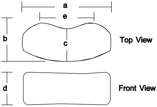
Figure 1. Geometry of vertebral specimens.
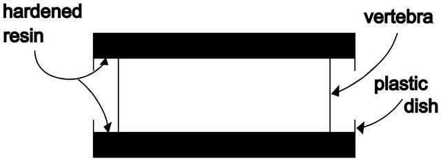
Figure 2. Vertebral test construct.
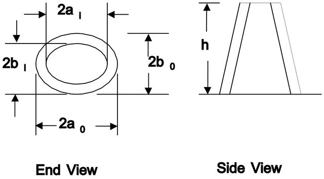
Figure 3. Distal radii wrist bone geometry.
3. MEASUREMENT AND TESTING RESULTS
3.1. Vertebrae
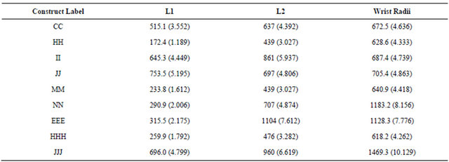
Table 1 lists the measurements of the geometric parameters shown in Figure 1 for the L1 and L2 vertebrae.
Table 2 lists the failure loads and the slopes of the nearly linear load/displacement relations obtained during the compression testings, for all 18 vertebral specimens.
3.2. Right Distal Radii
Tables 3 and 4 list the measurements of the parameters of Figure 3 for the distal and proximal ends of the right radii specimens, and also in Table 4 the specimen lengths.
Finally, Table 5 lists the failure loads and the slopes of the nearly linear load/displacement relations obtained during compression testing.
4. ANALYSIS
4.1. Vertebrae
To determine the vertebral strengths we needed to know their cross-section areas. To this end we used the geometry represented in Figure 1 together with the measured data listed in Table 1. To facilitate this we divided the vertebral cross-section region into three parts as in Figure 4 with circle segments representing the ends and the central region being a near rectangle.
Using standard handbook mensuration formulas [4] for the segment areas we were able to estimate the vertebral cross-section areas in terms of the measured dimensions of Figure 3. From the summary analysis of the Appendix we obtained the following area algorithm:
Let t be defined as:
 (1)
(1)
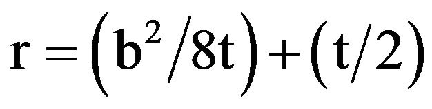
Next, let r be defined as:
 (2)
(2)
Then the cross-section area A of a vertebral specimen is approximately:
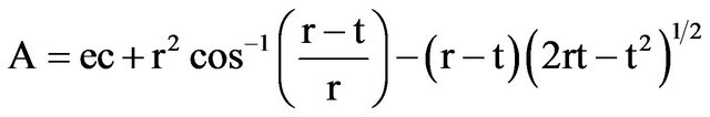 (3)
(3)

Figure 4. Segmentation of a vertebral cross-section area.
Table 1. Vertebral geometric measurements1 (see Figure 1).
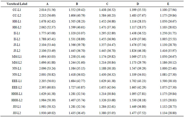
1Measurements are in inches (in) with millimeters (mm) in parentheses.
Table 2. Failure loads and stiffnesses of the 18 vertebral constructs.
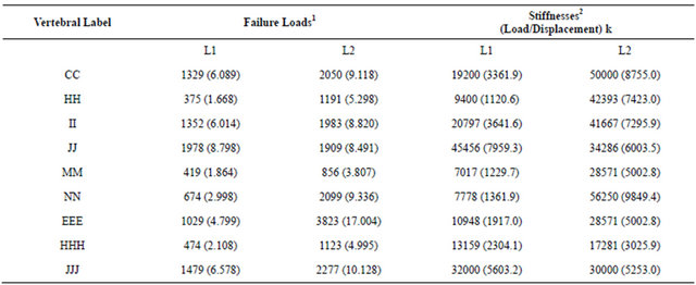
1Loads are in pounds (lb) with kiloNewtons (kN) in parentheses. 2Stiffnesses are in pounds per inch (lb/in) with kiloNewton per meter (kN/m) in parentheses.
where a, b, c, and e are shown in Figure 1. Once we have values for the cross-section areas, we can readily determine the specimen strength using elementary strength of materials formulas: Specifically, for a uniform cross-section member with length ℓ and cross-section area A, and subjected to a compressive load P as in Figure 5, the shortening δ of the member is simply:
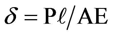 (4)
(4)
where E is the elastic modulus (see Beer and Johnston [6]).
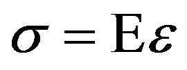
The stress and the strain ε are then defined as
Table 3. Distal end geometric measurements*.
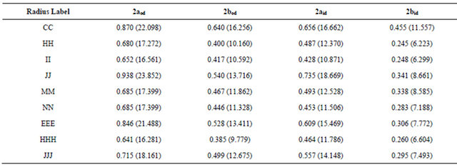
*Subscripts d for distal Measurements are in inches (in) with millimeters (mm) in parentheses.
Table 4. Proximal end geometric measurements* (see Figure 3).
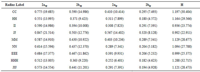
*Subscripts p for proximal. Measurements are in inches (in) with millimeters (mm) in parentheses.
Table 5. Failure loads and stiffnesses of the 9 right radii (wrist) constructs.

1Loads are in pounds (lb) with kiloNewtons (kN) in parentheses. 2Stiffnesses are in pounds per inch (lb/in) with kiloNewtons per meter (kN/m) in parentheses.
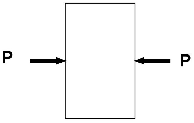
Figure 5. A specimen in compression.
 and
and 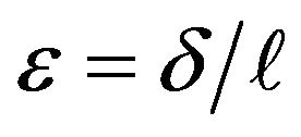 (5)
(5)
with the “strength” being the maximum stress value  occurring at the failure load
 , or at the collapse of the specimen member.
The elastic modulus E is a measure of the stiffness of the specimen. It is simply the slope k of the linear portion of a graphical representation between the stress σ and the strain ε, or equivalently, between the load P and the displacement δ. That is, from Eqs.4 and 5 we have
 or
or 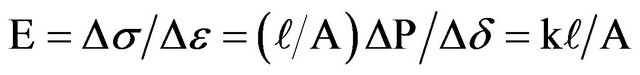 (6)
(6)
Where Δ is a finite difference.
The strength  and the stiffness E are thus measures of the structural integrity of the vertebral specimens and thus can be used for comparison evaluations.
4.2. Distal Radii
As with the vertebrae, we also needed the cross-section areas of the distal radii, to evaluate their strengths. To this end, consider again the sketch of the distal radii bone specimens shown in Figure 3. Although the specimens have a longitudinal taper, the measurements recorded in Tables 4 and 5 show that the taper is slight, so that for deformation and stress calculations it is reasonable to simply assume a linear cross-section area change.
The bone content of the radii cross-sections are nearly annular ellipses. Therefore, with an ellipse area being: , with a and b being semi-major and semi-minor axes, the distal and proximal cross-section areas are:
 (7)
(7)
The average bone cross-section is then
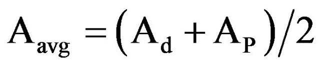 (8)
(8)
Consider again the side view of the radius specimen as in Figure 3 and as shown again in Figure 6 identifying the end areas and with an axial coordinate y. Then we see that the cross-section area A(y) along the axis of the specimen is:
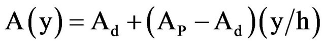 (9)
(9)
Beer and Johnston [6] state that the shortening δ of the tapered specimen is given by the formula:
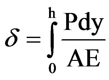 (10)
(10)

Figure 6. Distal radii wrist specimen geometry.
By substituting for A from Eq.9 we find δ to be:
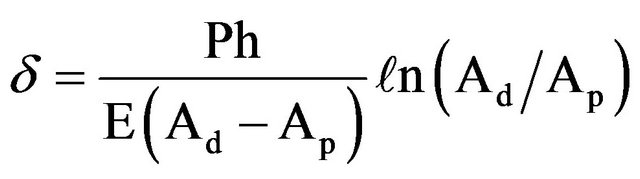 (11)
(11)
In the course of the loading of the specimen (before collapse) we found the loading and the deformation to be linearly related. That is,
 (12)
(12)
where, as with the vertebrae, the stiffness constant k may be identified as the slope of the newly linear load/displacement relation.
5. COMPUTED RESULTS
5.1. Vertebrae
Table 6 lists the cross-section areas of the L1 and L2 specimens, calculated using the formulas of Eqs.1-3, and the resulting strengths and elastic moduli.
We used the failure load data of Table 2 and the computed areas to obtain the strengths of the vertebrae. Also, by using the stiffnesses listed in Table 2 we obtained the elastic moduli using Eq.6.
5.2. Distal Radii
The radii strengths and elastic moduli can be computed using the failure loads and stiffness values listed in Table 6, the measured geometric dimensions of Tables 3 and 4, and then Eqs.7, 8 and 13, to determine the numerical results. To this end, it is helpful to initially determine the cross-section area parameters of Eqs.8 and 13.
In view of Eq.8, it is helpful to compute some area ratios needed for determining the elastic modulus. Also, it is useful to have the product of the construct height h (see Figure 3) and the stiffness k of Table 5. To this end Table 7 lists the distal, proximal and average areas and area ratios and stiffness-height products of the bone content of the various radii.
Finally, using failure loads listed in Table 5 and the parameters of Table 7, we obtain the radii strengths and elastic moduli as listed in Table 8.
6. DISCUSSION AND CONCLUSIONS
Table 9 summarizes the foregoing results providing a comparison between the strengths of the specimen constructs from the three sites. A glance at the results shows the general trend that there is a correlation between the strengths of the distal radii and the vertebrae for the corresponding cadavers. There is an especially strong correlation between the radii and the L2 vertebrae.
Observe also in Table 9 that the strengths of the wrist radii are generally higher than those for the vertebrae.
Table 6. Vertebral construct cross-section areas, strengths, and elastic moduli.
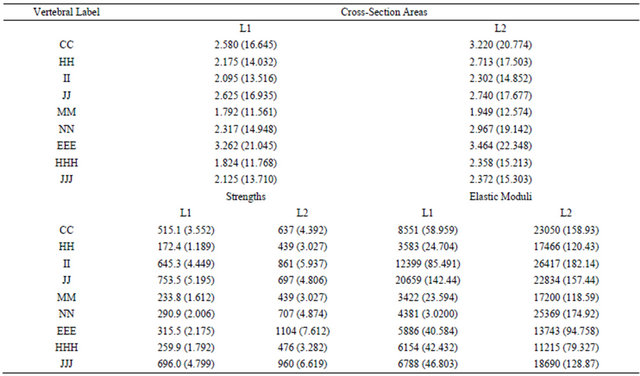
Values are in square inches (in2) with square centimeters (cm2) in parentheses, and in pounds per square inch (psi) with mega Pascals (mPa) in parentheses.
Table 7. Cross-section areas of distal radii bone, area ratios and stiffness-height products.
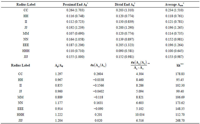
*Values are in square inches (in2) with square centimeters (cm2) in parentheses; **Units in reciprocal square inches (in–2); ***Units in pounds.
Table 8. Strengths and elastic moduli for the distal radii.
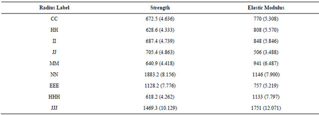
Values are in pounds per square inch (psi) with megaPascals (mPa) in parentheses.
Table 9. Strength comparisons for the three construct.
Values are in pounds per square inch (psi) with megaPascals (mPa) in parentheses.
This is to be expected since the radii bone is cortical whereas the vertebrae have load sharing between cortical and trabecular bone. Eswaran, et al. (2006) [7] discuss this effect in detail.
7. ACKNOWLEDGEMENTS
The authors acknowledge and appreciate the assistance of Richard Banto, Dale Weber, Y. Su, Susan Neuman, and Linda Levin.
REFERENCES
- National Institutes of Health (2000) NIH consensus development conference on osteoporosis.
- US Preventive Services Task Force (2011) Screening for osteoporosis: Recommendation statement. American Family Phyisican, 83, 1197-1200.
- Dimov, M., Khoury, J.D. and Tsang, R.C. (2010) Bone mineral loss during pregnancy: Is tennis protective? Journal of Physical Activity & Health, 7, 239-245.
- Oyen, J., Gjesdal, C.G., Brudvik, C., Hove, L.M., Apalset, E.M., Sulseth, H.C. and Hangeberg, G. (2010) Low-energy distal radius fractures in middle-aged and elderly men and women—The burden of osteoporosis and fracture risk—A study of 1794 consecutive patients. Osteoporosis International, 21, 1257-1267.
- Selby, S.M. (1972) CRC standard mathematical tables. 20th Edition, The Chemical Rubber Col, Cleveland. doi:10.1007/s00198-009-1068-x
- Beer, F.P. and Johnston Jr., E.R. (1992) Mechanics of materials. 2nd Edition, McGraw-Hill, New York.
- Eswaran, S.K., Gupta, A., Adams, M.F. and Keaveny, T.M. (2006) Cortical and trabecular load sharing in the human vertebral body. Journal of Bone and Mineral Research, 21, 307-313. doi:10.1359/jbmr.2006.21.2.307
APPENDIX
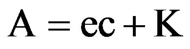
To establish a basis for Eqs.1-3, consider the circle segment in Figure A. From Reference [5] and/or other handbooks, the area K of the shaded region is:
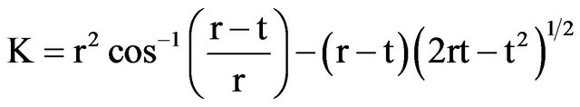 (A1)
(A1)
In view of the dimensions a, ···, e of Figure A, we immediately see that t and m are
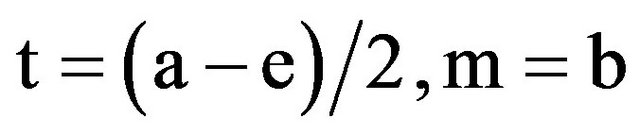 (A2)
(A2)
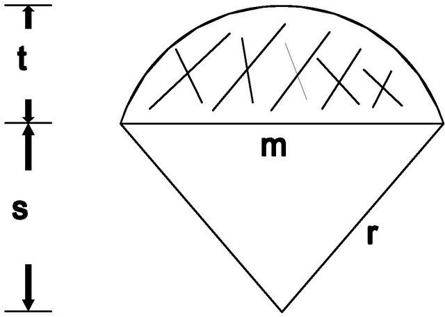
Figure A. Circle segment.
Also from [5] m, t, and r are related to each other by the expression:
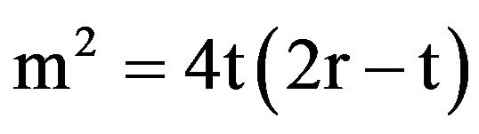 (A3)
(A3)
By solving for r we have
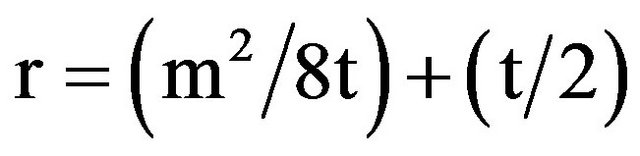 (A4)
(A4)
Referring again to Figure 1 and also to Figure 4 we see that the cross section areas A of the vertebral specimens may be represented as:
 (A5)
(A5)
or
 (A6)
(A6)
Eqs.A2, A4, and A6 form the basis for the algorithm of Equations.