Modern Economy
Vol. 3 No. 4 (2012) , Article ID: 21274 , 8 pages DOI:10.4236/me.2012.34049
Dynamic Model for Planning and Business Optimization
1Departamento de Ciências Básicas (ZAB), University of São Paulo at Pirassununga, Pirassununga, Brazil
2Faculdade de Engenharia (FAEN), Federal University of Dourados, Dourados, Brazil
3Departamento de Economia, Administração e Sociologia (LES), University of São Paulo at Piracicaba, Piracicaba, Brazil
Email: sergiodavid@usp.br, clivaldooliveira@ufgd.edu.br, derickdq@usp.br
Received April 5, 2012; revised April 15, 2012; accepted May 28, 2012
Keywords: dynamic systems; dynamic optimization; economic dynamics; mathematical modeling; rate of return; simulation; management strategy
ABSTRACT
The growing internationalization of markets, backed by the free movement of capital flows, has redefined the past quarter century’s business strategies and tends to continue driving economic and financial integration throughout this century. In this context, firms that aim to stand out in such markets should use the essence of the theoretical apparatus to allocate scarce resources efficiently. This means seeking the best possible benefits to offset the constraints that are inherent to the nature of the business environment. In this turbulent and competitive world, there is an increasing need to devise planning models to address the multiple issues that affect competitiveness, such as: planned rate of return, price adjustment, technological obsolescence, optimal investment path, among others. In an effort to contribute to solutions for this need, this paper proposes a dynamic model based on the Hamiltonian approach that combines the Cobb Douglas function and Pontryagin conditions. The model also suggests valuable improvements for company operations.
1. Introduction
In today’s tumultuous world with its scenario of complex interrelated variables and its intense uncertainties, corporate strategies must be unfailingly dynamic. Hence, constant readjustments are fundamental in dealing with the cyclical dynamics of self-regulated markets. Today, strategy and modeling cannot be taken as absolutes, for there are countless uncertainty factors that may be very difficult to resolve. The importance of business strategies and modeling of action planning increases in proportion to increasing uncertainty. Strategies must therefore be dynamic and change constantly to deal with unpredictable external factors. In view of the above, we believe that the best way to face today’s business uncertainties is through strategizing and modeling, followed by continuous revisions of the strategy and the model.
Established companies should brace themselves for a future of hypercompetition and be prepared to respond to rapid changes in the business environment by adopting a new approach—one that combines modeling and strategic thinking.
One of the basic notions in economics is that a company’s capital accumulation is a future-oriented activity, and as such, it should depend on what the company believes is likely to occur. The fact that the future cannot be known with certainty has led to several investigations of the effects of increased uncertainty on the company’s decision-making ability. Nickell [1], for instance, examined these effects based on several assumptions.
During the last forty years it has been increasingly recognized that many economic problems can be viewed as involving the optimization of an intertemporal objective function by a decision-maker who is constrained by a dynamic system subject to various kinds of uncertainties [2]. Robinson and Lakhani [3], demonstrated the fact that dynamic price models can be used to test the long run consequences of specific pricing rules or to determine the optimum long run pricing scenario within the context of any constraints which a manager might wish to impose. As opposed to the conventional static theory which emphasizes the instantaneous profit flow, the dynamic models use an appropriately discounted accumulated profit as the major parameter for making value judgments. They considered a specific example that emphasizes the importance of these ideas for a growth market and suggests that dynamic models can lead to as much as an order of magnitude more profit in the long run than the conventional static theory.
However, such problems arise both on the level of the individual firm, necessitating extensions of operations research and management science to methods of dynamic optimization [4] under uncertainty, as well as on the level of policy-making for national economy [2,4].
The field of economics and its priorities for analysis are broadened considerably leaving behind a monist view of the economy, as in the dominant model of economic analysis, and adopting a pluralist view where different forms of enterprise—each with its own form of governance and profit or surplus distribution and its own objectives—coexist, cooperate and compete in the economic system. In a plural economy approach, the forms of private enterprise that do not maximize profits and whose behavior logic is not guided by the capital factor, such as the various forms of SE (Social Economy) enterprises, no longer occupy a marginal position but are at the centre of economic analysis [5]. In accordance to [5], the field of economic analysis needs to be broadened, abandoning the mainstream monism that emphasizes the study of capitalist private enterprises and taking a plural view of the economy.
Moreover, in the globally competitive business world there is an increasing need to create planning models to deal with a wide variety of problems [6].
Regarding the method for the assessing and the planning the technology, Claro et al. [7] proposed a method, developed with the integration and adaptation of a set of state-of-the-art tools and concepts which involves, among others, dynamic planning and valuation and dynamic business plan preparation. Furthermore, Graves et al. [8], developed a new model for studying requirements planning in multistage production-inventory systems. Their approach is to use a model for a single production stage as a building block for modeling a network of stages and to analyze the single-stage model to determine the production smoothness and stability for a production stage and the inventory requirements. Also, the model attempts to show how to optimize the tradeoff between production capacity and inventory for a single stage.
However, do not have a tangible way to meet those terms.
We believe that there is an increasing need to devise planning models that address multiple issues which affect competitiveness, such as planned rate of return, price adjustment, technological obsolescence, and optimal investment path, among others.
In an effort to contribute to solutions to satisfy this need, we propose a dynamic coupled model that addresses the aforementioned issues. The model is based on a mathematical formulation using the Hamiltonian approach [9] considering the Cobb Douglas function and Pontryagin’s minimum principle. The Pontryagin’s minimum principle and the “minimum-time” problem were also used and derived by Lewis in optimal control applications involving the problem adjustment time in monetary growth model [10]. In this present work, the model is intended for application in environmental business action planning and we believe that this paper offers a contribution to this investigation field. It is divided as follows: Section 2 outlines the dynamic optimization model considering the Cobb Douglas function and Pontryagin’s conditions. Section 3 describes the conditions for optimality. Section 4 presents the results of simulations. Lastly, section 5 offers a discussion, our conclusions and a future outlook.
2. The Dynamic Optimization Model
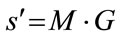
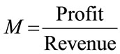
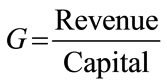
The development of a business must include a planned rate of return. Once the rate of return is determined, it can be written as a product of the profit margin vs. circulation of capital, as expressed by the following equation:
 (1)
(1)
where,
 (2)
(2)
and
 (3)
(3)
With this fact in mind, we examine the behavior of the rate of return (ROR) more closely. This close scrutiny reveals why the ROR does not follow its predicted course, and indicates how to change its course, or planning, depending on the type of business in question.
In addition, the model allows one to observe the optimal investment path, on both the finite and infinite horizons (steady-state values). In the case of the finite horizon, in particular, the model is more qualitative than quantitative. However, in both cases, it allows for a variety of sensitivity analyses.
The study involved two types of input market structures: an input market representing imperfect competition (convex adjustment costs) and a market of scale economies (concave adjustment costs) [11,12].
The cumulative profit to be maximized is then [13, 14]:
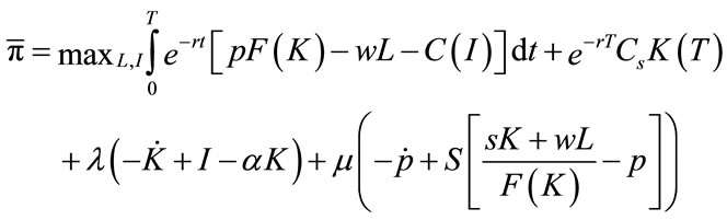 (4)
(4)
Equation (4) describes the company’s instantaneous cash flow constraints:
 (5)
(5)
 (6)
(6)
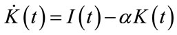
Factors K and L are the two input factors, i.e., capital stock and labor stock, respectively. The  function is the time derivative of K(t).
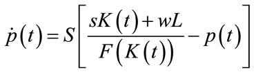
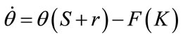
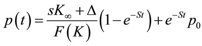
The  function is the unit price. The
  function is the time derivative of p(t) and states the price adjustment mechanism [9].
As an initial assumption, due to the minor variation in the value of L (number of employees), L is considered constant and can therefore be written as , while F depends only on K.
The F function can be seen as the Cobb Douglas function [15,17]. Thus,
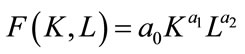 (7)
(7)
is the firm’s production function.
Since L is a constant value, one has , with
  and,
and, .
.
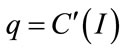
We also considered I(t) as the gross investment and C(I) as the total cost investment function, with
 and C(0) = 0.
The remaining parameters are as follows:
• π is the cumulative profit;
• w is the wage rate;
• Cs is the scrap value of the capital goods;
• S is a speed for price adjustment;
• r is the discount rate;
• α is the depreciation rate;
• ![]() is the capital return rate,
is the capital return rate,  , Ca is the unit value of the capital goods, and p is the annual profit.
We know that
 (8)
(8)
Thus, ![]() can be written as:
can be written as:
 (9)
(9)
Therefore,
 (10)
(10)
where
 (11)
(11)
We would like to point out that, in this context, the meanings of equations (6) and (10) are not regulated [15], but there is a planned objective for profit. Thus, it can be demonstrated that, under particular conditions, equations (6) and (10) are equivalent.
After some manipulation, Pontryagin’s necessary conditions yield:
 (12)
(12)
 (13)
(13)
 (14)
(14)
where  and
and  are the shadow prices related to K(t) and p(t) respectively.
With regard to the input market (suppliers), two conditions can be stated [6,16].
2.1. Convex Total Investment Costs
The supplier market is an imperfect capital market, where  and C(I) is assumed to be:
C(I) = A·I2 + B·I, A and B positive constants.
2.2. Concave Total Investment Costs
In this case, the costs decrease due to scale economies.
Therefore  and
and  where A is a positive constant. The problem here is a non-convex one. According to [5], it is possible to solve the artificially “convexified” problem by replacing the C(I) function with a function constructed by setting
  for all I,
  , where
 .
.
Thus, for this “convexified” problem,  is a feasible steady-state with a level of investment
  and an average cost of investment
![]() .
.
3. Conditions for Optimality
In addition to the conditions stated in the previous section, several important conditions for the model’s application and for investigation are considered in this section, namely: planned ROR, price adjustment and optimal investment path, technological obsolescence involving a depreciation model and various general conditions.
3.1. Planned Rate of Return
This model works with a planned ROR. Therefore, ![]() is a planned objective of the company. For instance, if the objective is to achieve a ROR of 12%, the model maximizes the cumulative profit for this kind of premise. In addition, one can write:
is a planned objective of the company. For instance, if the objective is to achieve a ROR of 12%, the model maximizes the cumulative profit for this kind of premise. In addition, one can write:
 , where
  (profit margin) and
  (circulation of capital).
If ![]() changes, s also changes because
changes, s also changes because . Thus, it is possible to evaluate the two effects separately to achieve the same
 ![]() value. In some situations it is better to vary M and in others it is more advantageous to vary G.
value. In some situations it is better to vary M and in others it is more advantageous to vary G.
3.2. Price Adjustment and Optimal Investment Path
The dynamics that governs the price is that of equation (10), based on the planned ROR (the company’s objective). Combining equation (10) with equation (1) and using a numerical technique to converge to a fixed point (which will be explained in greater detail in Section 4), the model leads the price and capital values to converge at an equilibrium point, indicating the optimal investment path.
3.3. Technological Obsolescence and Depreciation Model
The historical depreciation model is not the best one to explain technological obsolescence. Instead, technological obsolescence is best explained by the sum-of-digits model [17]. However, because the time between the several operation ages (vintages) [17-20] is extremely discrepant, it is more convenient to model depreciation as a general model based on the Fisher-Pry model (S shape model). Instead of a constant value of α, the depreciation rate has a time variation. The Fisher-Pry mathematical model can be written as:
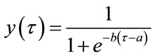 (15)
(15)
where y(t) is the fraction of the new technology in time t. The parameter a describes the time at which the new technology reaches 50% of the entire time between the new and the old technologies. The parameter b measures the speed of substitution. Based on the Fisher-Pry model, the mean depreciation rate can be written as:
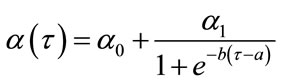 (16)
(16)
where α0 is the initial depreciation rate. The final depreciation rate is . Thus, equation (16) can be incorporated into the dynamic equations, keeping in mind that
 .
.
The Figure 1 shows the evolution of the depreciation rate.
3.4. General Conditions
The company is always constrained to satisfy demand and presumably knows all the relevant information about the supply and demand functions (output market, customers) [21,22]. The figure 1, show the depreciation rate. In this figure we can see a significant grow at the point 7.6 and at year 10 the depreciation rate is 3 times more.
Assuming a demand function p = a – bQ, the maximum revenue value occurs at point a/2b. Figure 2 indicates that a slight variation around the equilibrium point, assuming an admissible variation in p, causes a slight variation in Q = F(K).
This slight variation in Q causes a slight admissible variation in the revenue. The model exploits this range of variations because the solution depends on a type of contraction to a fixed point before converging to stationary values due to a numerical solution.
The Figure 2 illustrates the range of applications of the model. The upper portion of this figure contains the supply and demand functions. The red line corresponds to the supply function and the blue line to the demand function. In the lower portion of this figure, the green line corresponds to the revenue curve as a function of Q = F(K).
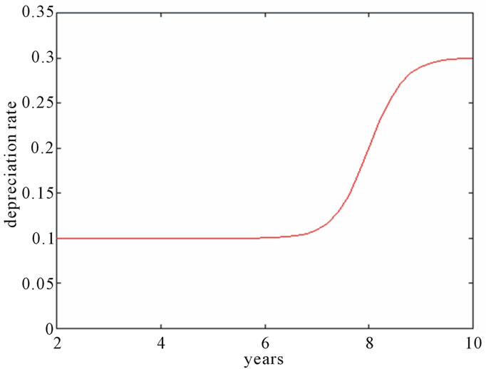
Figure 1. Depreciation rate evolution.
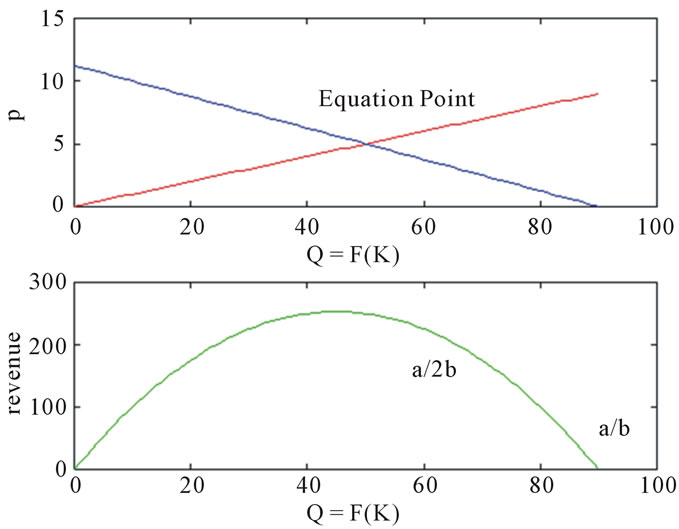
Figure 2. Range for model application.
4. Simulations Results
Assuming a fixed value of I(t), or equivalently, its infinite value, Equation (5) can be written as follows:
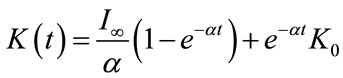 (17)
(17)
It is interesting to note that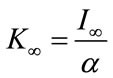 , as expected.
The model assumes the maintenance of I(t) as a t constant and calculates K= K(t) as a time function for each different time. Proceeding in the same way, equation (6) will become:
 (18)
(18)
The equations (19) and (20) can be treated similarly, but their integration constants must disappear over time. The time it takes for them to reach their stationary values can be investigated (this is a sort of “warm-up” time). Their stationary values will thus be:
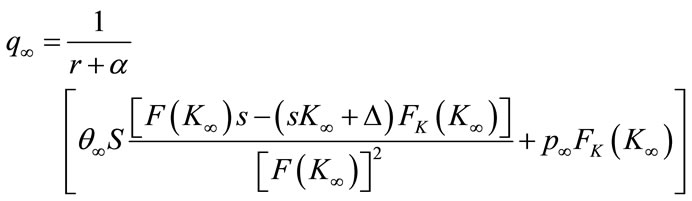 (19)
(19)
 (20)
(20)
The four equations (17)-(20) are then coupled and I(t) is calculated from equation (14) and with I(q) = (C'(Ì(q)))–1.
See the additional observation for concave adjustment costs as in [5].
The model is actually more qualitative than quantitative, but it gives a good idea about the optimal path and, in addition, it allows for a thorough sensitivity analysis.
The equations resulting from the Hamiltonian approach (12), (13) and (14) and the model’s equations (3), (6) and (10) were solved using the Matlab/SimulinkTM software package.
Next, we describe some of the [the most important] results of these simulations and briefly discuss each one.
The Figure 3 indicates, for the concave adjustment costs and rate of return , that the relation between profit margin (M) and capital circulation (G) has an important dependence about the depreciation rate. If the company, for instance, can not to make a higher capital circulation, the depreciation rate can not be increased.
The Figure 4 presents the phase diagram for the steady-state relative to depreciation rate equal to 0.1 and C(I) with the concave shape. Besides, it shows the in
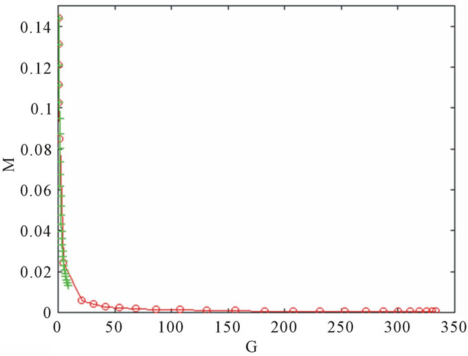
Figure 3. C(I)—concave shape.
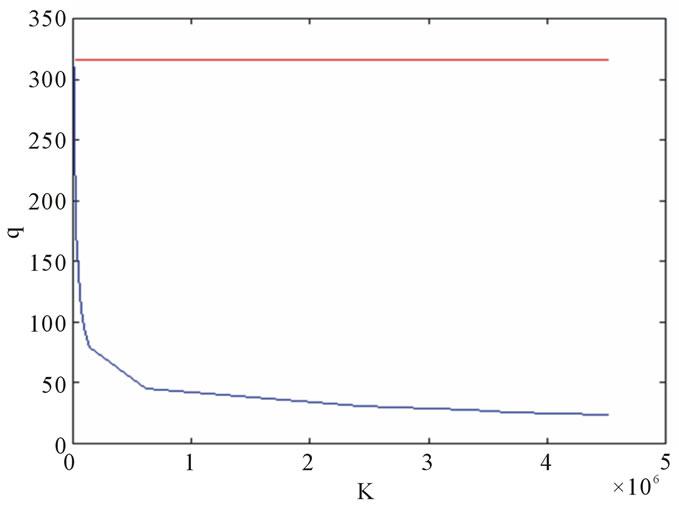
Figure 4. C(I)—concave shape.
vestment path to reach the feasible steady-state  for a given K0 value. The value for
  is 8346 and do not appear in figure because its scale values. Price variations achieved by changing the ROR are presented in Figures 5 and 6.
The Figures 5 and 6 shows that when the ROR increases, shifting the curve to the right and the relationship between M and G also changes.
Price variations achieved by changing the ROR are presented in Figures 7 and 8. At the figure 8, the ROR of the 12%, presents a discontinuity around 17 years.
The company can choose how to achieve a ROR of 18%. For instance, it can increase G or, alternatively, it can increase M between the admissible limits.
When the ROR ![]() changes from 12% to 18%, for instance, the price level goes to a higher steady-state value.
changes from 12% to 18%, for instance, the price level goes to a higher steady-state value.
The Figure 9 shows the phase diagram of Price (p) vs. Capital (K) for the cost convex shape, with ![]() = 12% and a depreciation rate of 0.1, that is the common values usually found in the literature. In this figure, note that the Price reaches the steady-state.
= 12% and a depreciation rate of 0.1, that is the common values usually found in the literature. In this figure, note that the Price reaches the steady-state.
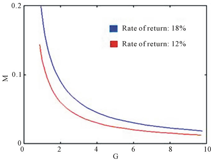
Figure 5. C(I)—convex shape.
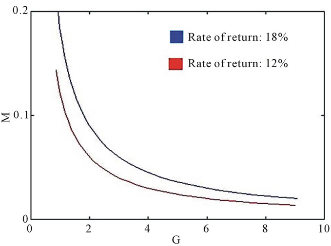
Figure 6. C(I)—concave shape.
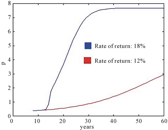
Figure 7. C(I)—concave shape.
On the other hand, Figure 10 shows the phase diagram of Price (p) vs. Capital (K) for a cost concave shape with ![]() = 18% and a depreciation rate of 0.3.
= 18% and a depreciation rate of 0.3.
The phase diagram in Figure 11 shows the cost con-
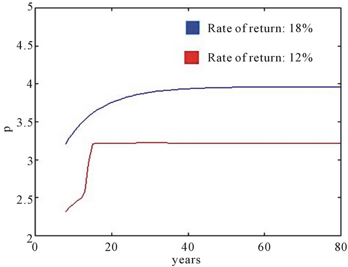
Figure 8. C(I)—convex shape.
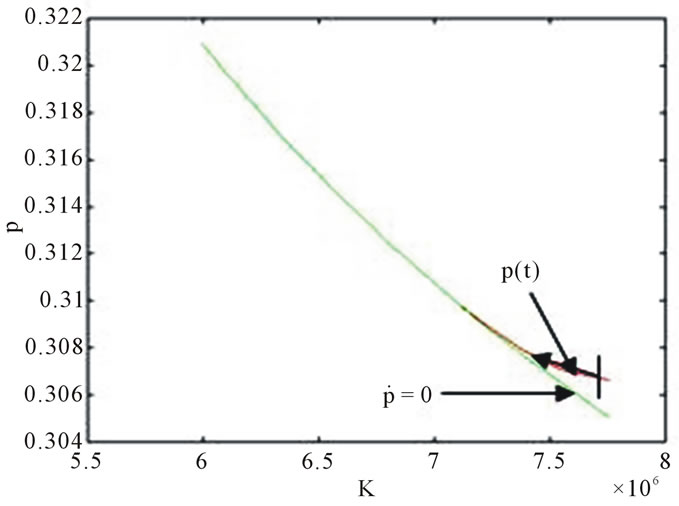
Figure 9. Phase diagram for C(I) convex shape.
vex shape and a depreciation of 0.1, as well as the investment path to reach the steady-state for a given K0 value.
The Figure 12 shows the phase diagram for a cost convex shape and depreciation equal to 0.3. A comparison of this figure with Figure 11 with the same value of K0 indicates that the steady-state was reached at a lower value. This implies a lower ROR at the equilibrium point.
5. Conclusions
An evaluation of the model’s variations of the steadystate price indicates that the concave cost model is more sensitive and therefore has a higher probability of leaving a given operating point stipulated by the company’s objective as the depreciation rate increases.
However, as the depreciation rate increases, two conditions can be observed in the model, i.e., an increase in the steady-state price and an increase in the circulation of capital (G), although the profit margin (M) may sometimes decrease. In fact, the best situation would be in-
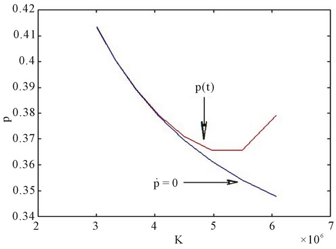
Figure 10. Phase diagram for C(I) concave shape.
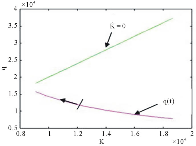
Figure 11. Phase diagram for C(I) convex shape and depreciation 0.1.
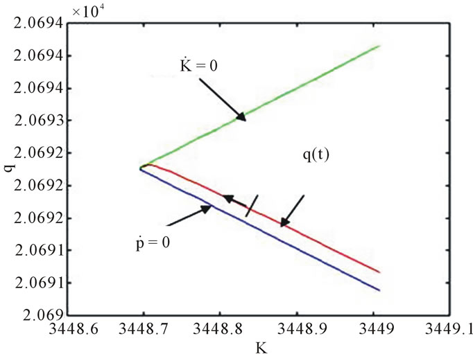
Figure 12. Phase diagram for C(I) convex shape and depreciation 0.3.
crease in G and M, but some companies have large amounts of capital and which they cannot easily put into circulation.
Another fact about our model is that the stationary point has a lower profit value, since the profit is given by the expression , where
 ![]() is the planned ROR and Ca is the value of capital goods.
is the planned ROR and Ca is the value of capital goods.
With the increase in ROR, ![]() , the main condition observed is a price increase. In certain cases, regulatory agencies may establish a maximum limit for prices (or tariffs), causing the planned ROR to become unattainable. Moreover, taking into account possible changes in the price (or tariff), another relevant issue is undoubtedly the competition (output market). However, a possible shift from the supply and demand operating point can be foreseen.
, the main condition observed is a price increase. In certain cases, regulatory agencies may establish a maximum limit for prices (or tariffs), causing the planned ROR to become unattainable. Moreover, taking into account possible changes in the price (or tariff), another relevant issue is undoubtedly the competition (output market). However, a possible shift from the supply and demand operating point can be foreseen.
A possible way to achieve greater accuracy and confidence in the model’s application, even for qualitative purposes, would be to make a data survey using regression and data fitting models, employing the two main functions involved: the Cobb-Douglas type F(K,L) function, and the production function (or F(K)), if it depends only on K and C(I). The same applies to total investment costs or adjustment costs.
This newly developed model is very comprehensive and allows for the evaluation of other types of parameters, such as the sensitivity of discount or interest rates, r, or variations in the cost of a capital good, Ca.
We believe that the use of this optimization model may make action planning clearer and lead to easier, more accurate and efficient decisions.
REFERENCES
- S. Nickell, “Uncertainty and Lags in the Investment Decisions of Firms,” The Review of Economic Studies, Vol. 44, No. 2, 1977, pp. 249-263. doi:10.2307/2297065
- J. Matulka and R. Neck, “Optcon: An Algorithm for the Optimal Control of Nonlinear Stochastic Models,” Annals of Operations Research, Vol. 37, No. 1, 1992, pp. 375-401. doi:10.1007/BF02071066
- B. Robinson and C. Lakhani, “Dynamic Price Models for New-Product Planning,” Management Science, Vol. 21, No. 10, 1975, pp. 1113-1122. doi:10.1287/mnsc.21.10.1113
- M. Alghalith, “General Closed-Form Solutions to the Dynamic Optimization Problem in Incomplete Markets,” Applied Mathematics, Vol. 2, No. 4, 2011, pp. 433-435. doi:10.4236/am.2011.24054
- R. Chaves and J. L. Monzón, “Beyond the Crisis: The Social Economy, Prop of a New Model of Sustainable Economic Development,” Service Business, Vol. 6, No. 1, 2012, pp. 5-26. doi:10.1007/s11628-011-0125-7
- J. C. Eckalbar, “Closed-Form Solutions to Bundling Problems,” Journal of Economics & Management Strategy, Vol. 19, No. 2, 2010, pp. 513-544. doi:10.1111/j.1530-9134.2010.00260.x
- J. Claro, et al., “Integrated Method for Assessing and Planning Uncertain Technology Investments,” International Journal of Engineering Management and Economics, Vol. 1, No. 1, 2010, pp. 3-30.
- S. C. Graves, et al., “A Dynamic Model for Requirements Planning with Application to Supply Chain Optimization,” Operations Research, Vol. 46, No. 3, 1998, pp. S35-S49. doi:10.1287/opre.46.3.S35
- E. G. Davis, “A Dynamic Model of the Regulated Firm with a Price Adjustment Mechanism,” The Bell Journal of Economics and Management Science, Vol. 4, No. 1, 1972, pp. 270-282. doi:10.2307/3003148
- S. D. Lewis, “Adjustment Time and Optimal Control of Neoclassical Monetary Growth Models,” Optimal Control Applications and Methods, Vol. 2, No. 3, 1981, pp. 251- 267. doi:10.1002/oca.4660020305
- L. E. Ohanian, E. C. Prescott and N. L. Stokey, “Introduction to Dynamic General Equilibrium,” Journal of Economic Theory, Vol. 144, No. 6, 2009, pp. 2235-2246. doi:10.1016/j.jet.2009.09.001
- R. Davidson and R. Harris, “Non-Convexities in Continuous-Time Investment Theory,” Review of Economic Studies, Vol. 48, No. 2, 1981, pp. 235-253. doi:10.2307/2296882
- E. Silberberg, “The Structure of Economics: A Mathematical Analysis,” 2nd Edition, McGraw Hill, Boston, 1990.
- H. Goldstein, C. P. Poole and J. Safko, “Classical Mechanics,” 3rd Edition, Addison Wesley, Boston, 2001.
- S. Katayama, “Optimal Investment Policy of the Regulated Firm,” Journal of Economic Dynamics and Control, Vol. 13, No. 4, 1989, pp. 532-552. doi:10.1016/0165-1889(89)90002-X
- E. P. López, et al., “A Model Predictive Control Strategy for supply Chain Optimization,” Computers & Chemical Engineering, Vol. 27, No. 8-9, 2003, pp. 1201-1218. doi:10.1016/S0098-1354(03)00047-4
- L. K. Vanston and R. L. Hodges, “Depreciation Lives for Telecommunications Equipment,” Technology Futures, Inc., Austin, 1996.
- S. L. Barreca, “Comparison of Economic Life Techniques,” Technology Futures, Inc., Austin, 1999.
- L. C. Won, “On the Policy Implications of Endogenous Technological Progress,” The Economic Journal, Vol. 111, No. 471, 2001, pp. 164-179. doi:10.1111/1468-0297.00626
- H. Aoyama, et al., “Fluctuation of Firm Size in the LongRun and Bimodal Distribution,” Advances in Operations Research, 2011, pp. 1-21. doi:10.1155/2011/269239
- R. Dorfman, “An Economic Interpretation of Optimal Control Theory,” American Economic Review, Vol. 59, No. 5, 1969, pp. 817-831.
- L. G. Epstein, “The Le Chatelier Principle in Optimal Control Problems,” Journal of Economic Theory, Vol. 19, No. 1, 1978, pp. 103-122. doi:10.1016/0022-0531(78)90058-3