Journal of Environmental Protection
Vol.08 No.02(2017), Article ID:74243,18 pages
10.4236/jep.2017.82012
Using Crop Management Scenario Simulations to Evaluate the Sensitivity of the Ohio Phosphorus Risk Index
Elizabeth A. Dayton1*, Christopher H. Holloman2, Sakthi Subburayalu1, Mark D. Risser2
1School of Environment and Natural Resources, The Ohio State University, Columbus, OH, USA
2Statistical Consulting Services, Department of Statistics, The Ohio State University, Columbus, OH, USA
![]()
Copyright © 2017 by authors and Scientific Research Publishing Inc.
This work is licensed under the Creative Commons Attribution International License (CC BY 4.0).
http://creativecommons.org/licenses/by/4.0/


Received: January 4, 2017; Accepted: February 17, 2017; Published: February 21, 2017
ABSTRACT
Phosphorus (P) risk indices are commonly used in the USA to estimate the field-scale risk of agricultural P runoff. Because the Ohio P Risk Index is increasingly being used to judge farmer performance, it is important to evaluate weighting/scoring of all P Index parameters to ensure Ohio farmers are credited for practices that reduce P runoff risk and not unduly penalized for things not demonstrably related to runoff risk. A sensitivity analysis provides information as to how sensitive the P Index score is to changes in inputs. The objectives were to determine 1) which inputs are most highly associated with P Index scores and 2) the relative impact of each input variable on resultant P Index scores. The current approach uses simulations across 6134 Ohio point locations and five crop management scenarios (CMSs), representing increasing soil disturbance. The CMSs range from all no-till, which is being promoted in Ohio, rotational tillage, which is a common practice in Ohio to full tillage to represent an extreme practice. Results showed that P Index scores were best explained by soil test P (31.9%) followed by connectivity to water (29.7%), soil erosion (13.4%), fertilizer application amount (11.3%), runoff class (9.5%), fertilizer application method (2.2%), and finally filter strip (2.0%). Ohio P Index simulations across CMSs one through five showed that >40% scored <15 points (low) while <1.5% scored >45 points (very high). Given Ohio water quality problems, the Ohio P Index needs to be stricter. The current approach is useful for Ohio P Index evaluations and revision decisions by spatially illustrating the impact of potential changes regionally and state- wide.
Keywords:
Ohio P Index, Sensitivity Analysis, P Index Simulations, RUSLE2 Simulations, Crop Management Simulations

1. Introduction
With 74,000 farmers, farming more than 10 million crop acres in Ohio, USA [1] agricultural phosphorus (P) runoff is a major environmental concern. Due to continued water quality concerns, the Ohio Lake Erie Phosphorus Task Force II Final Report [2] is calling for approximately a 40% reduction in P loading into the Western Lake Erie Basin (WLEB). The target reductions are based on a harmful algal bloom (HAB) projection model [3] using the correlation between P loading into the WLEB (March 1 to June 30) and subsequent HAB severity. Despite reductions in total P loading to Lake Erie [4] , the proportion as soluble P shows distinct increases [5] [6] .
In response to water quality concern, there is an increased emphasis on the use of state P indices in the recently revised USDA Natural Resources Conservation Service (USDA-NRCS) Practice Standard Code 590, Nutrient Management [7] [8] [9] [10] which considers both crop production and P runoff risk. Lemunyon and Gilbert [11] first introduced the P risk index approach as a qualitative estimate of P runoff risk based on field characteristics and farmer management practices. The Ohio Phosphorus Risk Index (P Index) is intended to provide a field-scale estimate of P runoff risk [12] . In Ohio there is an ongoing effort to evaluate and revise the Ohio P Index to ensure that P Index scores accurately reflect field-scale runoff risk. Typical of P indices [13] [14] [15] , the Ohio P Index [12] includes field specific P source and transport factors. Information regarding P source factors is provided by the farmer and includes soil test P (STP, Bray-P1 mg・kg−1), planned fertilizer/manure application amount and method of application. Key field specific P transport factors include erosion potential [16] , connectivity-to-water, based on proximity to intermittent or perennial streams and evidence of surface runoff and finally runoff class which considers the combined effect of hydrologic soil group with slope steepness. Each factor has an associated weighting/scoring based on its presumed contribution to P runoff risk. Comparing multiple state P Index weighting/scoring and interpretation for the same sets of field data has revealed substantial differences [13] [17] among state P indices. Ideally, weightings should be evaluated based on measured P runoff data [9] . Field work currently underway in Ohio should be able to better inform weighting/scorings as they are related to P loss. In the meantime sensitivity analysis is being used to investigate the relationship between Ohio P Index parameters and current Ohio P Index scores. Using sensitivity analysis to assess the impact these input parameters have on Ohio P Index scores will guide Ohio P Index revision efforts to ensure farmers will be credited for management practices that reduce P runoff risk and not unduly penalized for things not demonstrably related to runoff risk.
A sensitivity analysis can provide information as to how sensitive the final P Index score is to changes in inputs [18] [19] [20] [21] [22] . Sensitivity analyses have also been used to evaluate other nonpoint-source pollution models [23] [24] [25] [26] [27] [28] . Inputs that exert extreme influence on the final score should be prioritized for reevaluation, and field studies verifying the accuracy of the relationship between the inputs and final score can be designed in a way that provide the most power for testing those inputs. In addition, an understanding of sensitivity will allow farmers to prioritize changes to their management practices in order to reduce their runoff risk.
Typically sensitivity analyses use a deterministic or stochastic approach. A stochastic sensitivity analysis [19] [20] [22] , explores the effect of all input variables simultaneously, and is able to make statements regarding the effect of an individual variable while accounting for the effects of all other variables. A stochastic sensitivity analysis allows for the specification of a complete probability distribution for each input variable, as well as accounting for unexplained variability in the output variable [29] . A stochastic approach is able to account for correlation among the input variables, and can make overall statements about how an input variable impacts the output variable instead of being limited in scope to statements with respect to a baseline condition.
Unlike stochastic approaches, deterministic sensitivity analyses based on baseline scenarios have been shown to give results that vary depending on the baseline scenario chosen [30] . A deterministic sensitivity analysis [18] [19] [21] [31] explores the impact of each variable separately, by calculating a relative sensitivity when the particular variable of interest varies over some subset of its range of possible values while all other variables are fixed at a baseline or average level.
An earlier sensitivity analysis [22] evaluated Ohio P Risk Index inputs for five Ohio watersheds, using a stochastic approach. The range of several input parameters were estimated using uniform or triangular distributions or professional judgement. Building on the work of Williams et al. [22] , three sensitivity analyses, two using a stochastic approach were used to understand the relationship between each P Index parameter and the Ohio P Index scores using data from the entire population of interest across a broad range of crop management scenarios (CMSs) for all of Ohio, and evaluate the relationship between the components that make up the individual parameters and the P Index scores and one using a deterministic approach to evaluate the impact of each P Index parameter on the range of P Index scores is presented in the current study. The objectives of this study are to 1) determine the inputs to which the P Index scores are most sensitive, and 2) understand the degree to which individual P Index parameters can impact the range of P Index scores.
2. Materials and Methods
Our approach comprised a data generation phase and a data analysis phase. In the first phase, data were generated to create a representative distribution of P Index input parameters across the state of Ohio and five CMSs. These inputs were generated using a combination of stochastic data generation and logical selection of combinations of inputs. Having generated the data, the second phase proceeded by conducting statistical analysis of the simulated data and the final P Index scores derived from those data. The statistical analysis was conducted in three parts corresponding to their explanatory power and possible range of P Index score movement to the combinations based on two types of inputs. The two input types include the P Index parameter and the raw component inputs that contribute to the P Index parameter.
2.1. Data Generation
An overview of the Ohio P Index [12] worksheet, including P Index parameters, associated sub-value scoring/weighting and interpretation, is provided in Table 1. Sub-values for parameters are added together to determine a final P Index score. To obtain a representative spatial distribution of P Index input parameters for running P Index simulations across varying crop management scenarios (CMSs, Table 2), a random sample of 20,000 Ohio point locations was generated in ArcMap [32] . Point locations were filtered to remove those not designated as crop land (corn, soybeans and wheat) using the 2012 cropland data layer, at a 10 m raster resolution [33] resulting in 6134 point locations.
Crop Management Scenarios. Crop management scenarios (Table 2), re- presenting increased levels of soil disturbance for soybean/corn rotations, were chosen in consultation with Ohio USDA-NRCS personnel. The CMSs include all no-till, which is a practice being promoted in Ohio, rotational tillage, which is a common practice in Ohio to full tillage to represent an extreme practice (Table 2).
Erosion Potential. To compute the soil loss values and field residue cover at each point location, the dll version of the Revised Universal Soil Loss Equation [16] was used. Required RUSLE2 inputs including county, soil map unit, slope length, slope steepness were extracted from the gridded Soil Survey Geographic database (gSSURGO) data for Ohio available at a 10 meter raster resolution [34] . The representative slope length and steepness of the dominant (having the highest component percentage) soil series within each map unit was used at each point location. In addition to SSURGO inputs, RUSLE2 requires crop management inputs including yield goal (Table 2). A yield goal of 50 bu・A−1, for soybeans and 160 bu・A−1 for corn, was used for all crop management scenarios.
Connectivity to Water. The Ohio P index considers the presence or absence of runoff concentrated flow from a field as well as the field’s adjacency to an intermittent or perennial stream (Table 1) in determining connectivity to water sub-values. Because the distribution of these inputs is not known, a set of decision making criteria was established in consultation with Ohio USDA-NRCS personnel. The presence of a surface drain was presumed where hydrologic soil group was a C/D or D and slope was <1 percent. Similarly where hydrologic soil group was C/D or D and slope was >2 percent the presence of a defined waterway was presumed. A point locations’ adjacency to an intermittent or perennial stream was assigned based on a buffer distance of 250 m using National Hydrography stream Data [35] based on professional judgement in consultation with Ohio USDA-NRCS personnel.
Runoff Class. Runoff class sub-values at each point location were determined by extracting the representative percent slope steepness and hydrologic soil

Table 1. Ohio Phosphorus Risk Index (P Index) overview of parameters (Site Characteristic Line Items) with associated weighting or scores (sub-values) and interpretation. Sub-values are added together to determine the P Index score. Also, Ohio Phosphorus (P) Risk Index score categories and abridged interpretations.
Source: USDA-NRCS-OH (2001).
Table 2. Crop management scenarios (CMSs) used as inputs to the Revised Universal Soil Loss Equation Version 2 (RUSLE2) representing soybean/corn rotations with increasing levels of soil disturbance.
group from the gSSURGO data [34] and assigned to each point location based on the lookup table provided in the P Index [12] . If a point location had a dual hydrologic soil group, for example C/D (drained/un-drained condition), the drained condition C was used as input.
Soil Test Phosphorus. Soil test P (STP) values were randomly selected from a distribution of possible STP values derived from data provided by the three largest soil test laboratories servicing Ohio (A & L Great Lakes Laboratories, Brookside Laboratories Inc, and Spectrum Analytic) at a zip code resolution. All STP (>500,000) values from 2009 to 2012 were candidates for use in the sensitivity analysis. Possible values ranged from 1 to 4172 mg・kg−1 Bray-P1. However across 88 Ohio counties the 50 percentile ranged from 6.3 to 131 mg・kg−1 Bray-P1. A STP value was randomly drawn from all values within the same sub-basin (USGS Hydrologic Unit Code-8) as the point location.
Fertilizer Application Amount. Fertilizer application amount was determined for the rotation based on the Tri-State Fertility Guidelines [36] using the assigned STP level and corn/soybean yield goal.
Fertilizer Application Method. The fertilizer application method sub-value is based on whether or not fertilizer is applied, time until applied fertilizer is incorporated and/or the amount of field cover at the time of application (Table 1). A combination of random selection and deterministic selection was used for each of the 30,670 combinations of 6134 point locations and five crop management scenarios. Field cover was determined from RUSLE2 [16] output based on a fall (Nov. 17) fertilizer application in crop year 1. If the application amount was zero (corresponding to a STP ≥ 40 mg・kg−1 Bray-P1), the application method sub-value is zero as well. If the fertilizer application amount was greater than zero, the amount of field cover was examined to determine candidate values of application method, and one of the candidate values was selected based on a random selection of time until incorporation (Table 1). If field cover was greater than 80%, the only candidate application method sub-value was 0.75. If fertilizer was applied and field cover was <80% but ≥50%, the candidate sub- values were 0.75 and 1.5. If field cover was <50% but ≥30%, the candidate sub-values were 0.75, 1.5, and 3.0. If field cover was <30%, the candidate sub-values were 0.75, 1.5, 3.0, and 6.0.
2.2. Data Analysis
The sensitivity analyses were performed using a Monte Carlo approach in which P Index values were simulated for a variety of field conditions in Ohio agriculture. All data simulation was performed using the R language and environment and was coded from scratch [37] . One simulated set of inputs (and, consequently, one final P Index score) was generated for each of the 30,670 combinations of 6134 point locations and five crop management scenarios. Where possible, the value of each input parameter was generated stochastically from available data. Where that was not possible, decision making criteria, as previously discussed, were used to establish a distribution of possible input values. Though weightings in the P Index are slightly different for fertilizer and manure application rate and method (Table 1), for simplicity only fertilizer input weightings have been shown here. Having generated simulated P Index scores for the 6134 point locations across five CMSs, we proceeded to perform three sensitivity analyses.
Analysis I, Sub-Value Contribution. The first stochastic sensitivity analysis examined the relationship between the P Index parameter sub-values and the final score. A linear regression was constructed using the final P Index score as the dependent variable and each sub-value as independent variables. Type III Sums of Squares was used to quantify each input’s explanatory power. Across all inputs, the Type III Sums of Squares were normalized to sum to 1 to provide a simple measure of relative explanatory power for each input.
Analysis II, Raw Component Contribution. The second stochastic sensitivity analysis examined the relationship between raw component inputs and crop management practices and the final P Index score. This analysis differs from the previous analysis in that raw component inputs and crop management practices are used as the independent variables rather than parameter sub-values. As with the parameter sub-value analysis a regression model was fitted to the data and the Type III Sums of Squares were used to estimate explanatory power for each of the characteristics.
Analysis III, Sub-Value Potential Impact. While the normalized Sums of Squares provide information about the unique explanatory power of each variable, they do not provide information about how much influence each sub-value can have on the final P Index score. Following Brandt and Elliot [18] , we performed a third analysis to quantify the amount the final P Index score can be changed by varying a single parameter. This deterministic sensitivity analysis used the same stochastic output used in the previous analysis of explanatory power. We first obtained a central P Index score (15.29), calculated by setting all sub-values at their average level. Next, we calculated the 2.5th and 97.5th percentiles of each sub-value. This range of values was used to represent a reasonable range of sub-values, excluding some potential outliers that might unduly impact the results. Next, we multiplied each regression coefficient from the previous analysis by its corresponding 2.5th and 97.5th percentiles of the sub-values to determine the range of score movement. For some inputs, the result is known beforehand and this analysis provides no useful information. For continuous variables and for some categorical scales, this second analysis provides some insight into how much impact a variable can have across a reasonable range of values for the input variable.
3. Results and Discussion
Erosion Potential. Increased levels of soil disturbance, resulting from increasing tillage across the CMSs, resulted in increased erosion. The percent frequency of erosion results of <2.24 Mg・ha−1・y−1 (<1 t・ac−1・y−1), 2.24 to 4.47 Mg・ha−1・y−1 (1 to 2 t・ac−1・y−1), 4.48 to 6.71 Mg・ha−1・y−1 (2 to 3 t・ac−1・y−1) and >6.72 Mg・ha−1・y−1 (>3 t・ac−1・y−1) are shown in Figure 1(a). Both no-till soybeans/corn but with a single
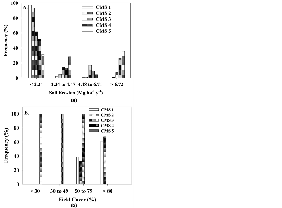
Figure 1. Frequency distribution of (a) soil erosion and (b) field cover, from RUSLE2 output for point locations across crop management scenarios (CMSs).
(CMS1) or double (CMS2) disk opener on the soybean planter, had similar low erosion levels with 97.1% and 93.2% of point locations having <2.24 Mg・ha−1・y−1 respectively. For other CMSs, erosion levels were distributed across the erosion classes <2.24 to >6.72 Mg・ha−1・y−1 (Figure 2). The Ohio P Index attributes 1 point per t・ac−1・y−1 soil loss. Results of simulations show that, except at extreme levels of tillage or slope steepness, soil loss was generally <2 t・ac−1・y−1.
Running RUSLE2.dll simulations across Ohio point location using appropriate gridded SSURGO [34] inputs and a range of crop management scenarios should better represent the range of erosion potential than earlier work [22] where erosion potential was estimated using “professional knowledge” and the average slope steepness, 5.4% for Great Miami River, 5.06% for Little Miami River, 11.98% for Scioto River, 2.78% for Upper Wabash and 1.80% for Western Lake Erie Basin, for specific Ohio watersheds.
RUSLE2 outputs for field cover, which are used in the determination of fertilizer placement method are presented in Figure 1(b). Across the CMSs, results show decreased field cover with increased soil disturbance. The proportion runoff total P that is particulate bound needs to be evaluated with field studies to determine the weighting to be sufficiently protective from a runoff P standpoint [11] . Runoff P measurements [38] indicated that runoff sediment accounted for 78% of runoff total P.
Connectivity to Water. Based on the decision making criteria, established with Ohio USDA-NRCS personnel, approximately 28% of point locations are presumed to have concentrated surface flow leaving the field. Defined waterways account for approximately 13% and surface drains 15% of the concentrated flow. Additionally, approximately 12.4% of point locations were considered adjacent (≤250 m) to an intermittent or perennial stream. Approximately 60% of P Index connectivity to water sub-values were 0 while 8.5%, 28%, 3% and 1% of sub- values were 4, 8, 12 and 16 points.

Figure 2. Fertilizer application method sub-values across crop management scenarios (CMSs).
Runoff Class. Approximately 66% of point locations are in the C hydrologic soil group with other hydrologic soil groups having a percent occurrence of 2 (A), 17 (B) and 16 (D). Runoff class sub-values for the point locations ranged from 0 to 15 with a sub-value of 4 having the highest frequency of occurrence at approximately 31%. Approximately 32% of runoff class sub-values are <4, while 37% are >4.
Soil Test Phosphorus. Following the Tri-State Fertility Guidelines [36] , 17.2% of point locations had Bray-P1 STP in the build-up range (<15 mg・kg−1 Bray-P1), while 35.8% had STP in the maintenance range (15 to 30 mg・kg−1), 14.8% of STP were in the drawdown range (30 to 40 mg・kg−1) and 32.2% had STP >40 mg・kg−1 indicating no additional P fertilizer should be applied.
Fertilizer Application Amount. Fertilizer application amount was determined based on Tri-State Fertility Guidelines [36] using the randomly selected STP and yield goal. Fertilizer application amount decreased as Bray-P1 STP increased with zero fertilizer application beyond 40 mg・kg−1 Bray-P1.
Fertilizer Application Method. A frequency distribution of fertilizer application method sub-values across CMSs is presented in Figure 2. Fertilizer placement method scores are highly impacted by field surface cover (Figure 1(b)), regardless of incorporation. This is evident in the fertilizer placement scores (Figure 2). The presumption is that surface cover will reduce P runoff. This presumption needs to be investigated in order to evaluate the P Index weighting for this parameter.
Ohio Phosphorus Risk Index Scores. A frequency distribution of Ohio P Index scores across crop management scenarios is presented in Figure 3.
The increase in P Index score due to crop management scenario is apparent and is a result of increased soil disturbance and decreased field cover. Increased soil disturbance increases erosion potential while decreased field cover increases both erosion potential and possible fertilizer placement method sub-values. Across the crop management scenarios, one through five, respectively, the current

Figure 3. Frequency distribution of Ohio P Index scores across crop management scenarios (CMSs).
study found that, 64.0%, 63.0%, 57.6%, 51.1%, and 40.7% scored <15 points (low); 35.1%, 36.0%, 40.6%, 45.7%, and 52.3% scored 15 to 30 points (medium); 0.65%, 0.67%, 1.42%, 2.66%, and 5.73% scored >30 to 45 points (high); while only 0.29%, 0.29%, 0.39%, 0.57%, and 1.24% scored very high or >45 points (Figure 3).
The current approach of evaluating Ohio P Index scores using simulations across a wide range of CMSs, a spatial distribution of point locations and running the RUSLE2.dll, provides improved soil erosion estimates as well as calculated field cover, resulting in a refinement of earlier work. The P Index scores in the current study are considerably lower than those reported in Williams et al. [22] where 65% to 76% of P Index scores were medium and between 88% and 95% of scores were within the medium and high risk categories. Contributing to these discrepancies are considerably higher connectivity to water sub-values due to the modified uniform probability distribution Williams et al. [22] used assigning 4% of sub-values as zero and 24% each to other possible sub-values of 4, 8, 12 and 16 points. While still an estimate, following the language in the P Index, which evaluates presumption of concentrated flow first and subsequently considers adjacency to intermittent or perennial streams, and the decision making criteria developed with Ohio NRCS personnel the current study estimated 60% of P Index connectivity to water sub-values were 0 while 8.5%, 28%, 3% and 1% of sub-values were 4, 8, 12 and 16 respectively. Runoff class sub-values were also higher in Williams et al. [22] possibly due to high estimates of average Ohio watershed slope steepness values (1.80% to 11.98%) used. In the current study runoff class sub-values were assigned based on point location representative slope steepness (median 1%) and hydrologic soil group and ranged from 0 to 15 with a sub-value of 4 having the highest frequency of occurrence at approximately 31%. The seemingly high estimates of average slope steepness [22] may also have inflated estimates of erosion potential. Across the five CMSs used in the current study 97.1%, 93.2%, 61.4%, 51.5% and 31.7% had soil loss <2.24 Mg・ha−1・y−1. Additionally assigning fertilizer application method sub-values based on a uniform probability distribution [22] probably results in an overestimation. In the current study a fertilizer application method sub-value of zero was assigned to 32.2% of point locations based on no fertilizer application (STP > 40 mg・kg−1). Further, based on field cover, it is not possible to have a uniform distribution of fertilizer placement method across a broad range of farmer management.
Statistical Analyses. The first (sub-value) and second (raw component) assessment (Table 3) of the sensitivity analysis quantified the unique explanatory power of each sub-value or raw component input. The regression analyses of the P Index parameter sub-value and raw component inputs (Table 3) produced remarkably similar results. In both analyses STP had the largest percent explanatory power with 31.9% in the sub-value analysis and 36.5% in the raw component analysis. In the sub-value analysis, connectivity to water had the 2nd highest explanatory power at 29.7%. Similarly the 2nd and 3rd highest explanatory
Table 3. Results of sensitivity analyses for Ohio P Index sub-values (line-item) as well as raw component inputs with their corresponding P Index parameter.
power in the raw component analysis were two components of connectivity to water, slope steepness (19.1%) and concentrated flow (24.4%). However, adjacency to an intermittent/perennial stream, also a component of connectivity to water, contributed only 4.6% explanatory power. This suggests that a presumption of concentrated flow and slope steepness rather than stream adjacency strongly influenced the connectivity to water sub-value. Slope steepness is also a component of erosion potential and runoff class, which may also contribute to its high explanatory power. In the sub-value analysis erosion had the 3rd highest explanatory power at 13.4%. Of the components of soil erosion in the raw component analysis, slope steepness had the greatest explanatory power (19.1%), while slope length (0.1%), soil erodibility (0.0%), rainfall erosivity (0.2%), crop management (0.4%), soil texture (0.0%), and residue cover (0.1%) contributed little. In the sub-value analysis, fertilizer application amount provided the 4th highest explanatory power at 11.3%, and was similarly moderate at 6% in the
raw component analysis. The 5th highest explanatory power in the sub-value analysis was runoff class (9.5%). Components of runoff class, slope steepness and hydrologic soil group, had explanatory power of 19.1% and 3.6% respectively, in the raw component analysis. Fertilizer application method provided the 6th highest explanatory power (2.2%) in the sub-value analysis. Similarly, in the raw component analysis the components of fertilizer application method field cover and fertilizer incorporation/timing had explanatory powers of 0.1% and 2.4%. Considering the abundance of work [39] - [47] showing the relationship between fertilizer/manure application method and runoff P risk, this result shows this P Index parameter may considerably under-weighted.
The third investigation evaluates the potential impact of each parameter on the range of P Index score are illustrated as a tornado plot (Figure 4) following Brandt and Elliot [18] . The results show the potential point range in P Index score movement (Figure 4) for each parameter: connectivity to water (12), STP (10), fertilizer application amount (9), soil erosion (8), runoff class (7), fertilizer application method (6) and filter strip (2).
While results from the two types of sensitivity analysis may appear to be inconsistent, they are actually providing different pieces of information. The first two analyses, focusing on explanatory power, give insight into which inputs are actually strongly associated with final P Index scores across the range of field conditions and CMSs. In contrast, the third analysis, focusing on potential influence of each input on the range of final P Index score, gives the hypothetical influence of each input across its observed range. In cases where the actual distribution of an input was highly skewed, it often had explanatory power lower than would be suggested by its potential influence. As an example, the parameter for fertilizer application amount has approximately one third the explanatory power of soil test phosphorus, but its range of impact is comparable to that of soil test phosphorus (Table 3 and Figure 4). When the range of each of these

Figure 4. Range in potential Ohio P Index score movement by varying a single parameter.
two variables is multiplied by the weights (to obtain potential influence), the values are approximately the same. However, the highly skewed distribution of scores for fertilizer application amount means that it is not highly correlated with final P Index score. As a result, its explanatory power is low despite its large potential for influencing the final P Index score. For example fields that have applied fertilizer can have their P Index score impacted highly. However, 32.2% of fields receive a score of zero for both fertilizer application amount and method due to STP > 40 mg・kg−1 and therefore their P Index score is highly impacted. Taking into account these differences should assist with appropriate re-weight- ing of Ohio P Index parameters.
Soil test P accounted for a high degree of explanatory power on the final P Index score (31.9%), however, following the Tri-State Fertility Guidelines fertilizer application amount only accounted for 11.3% of explanatory power. Based on the agronomic approach used 32.2% percent of point locations allowed for no P applications, however, in the current P Index, there is no actual prohibition against additional P application until a very high (>45 points) score is reached. This illustrates that, currently, for Ohio, the P Index approach could be perceived as less restrictive with regards to P application than an agronomic approach [8] [9] . For example under the current Ohio P Index weighting a Bray-P1 STP of 150 mg・kg−1 would result in only 10.5 points. Because that level of STP would require no further P additions, resulting in a sub-value score of zero for both fertilizer placement amount and method, it is not unlikely that this field could fall in the low risk category. Ongoing field P loss studies in Ohio will provide information to evaluate STP levels and P Index weightings as related to P runoff [48] - [52] .
Slope steepness, an integral part of connectivity to water, soil erosion and runoff class which ranked 2nd, 3rd and 5th in the sub-value sensitivity analysis, had the 3rd highest explanatory power (19.1%) in the raw components analysis and was responsible for the 2nd highest potential range of P Index score movement. Even though soil erosion had the 3rd highest explanatory power in the sub-value analysis, crop management, which is an integral part of soil erosion, had very little explanatory power in the raw component analysis. In fact, slope steepness seems to have had a greater contribution to soil erosion. For example (Figure 4) shows there are large differences in erosion within CMSs while Table 3 shows slope steepness having greater explanatory power than CMS. Hence the impact of crop management and slope steepness on soil erosion and subsequent P Index score needs to be carefully considered for P Index revisions, especially since farmers cannot control slope steepness. Soil erosion and runoff class sub- values increase with increasing slope steepness. However connectivity to water sub-values increase at both, high or low slope steepness due to the presumption of concentrated flow of runoff water leaving the field. Perhaps evaluating changes in RUSLE2 erosion results across not only changes in CMS, but also across slope steepness would be useful. While connectivity to water and STP ranked highest in the second sensitivity analysis, fertilizer application amount and soil erosion also played important roles.
4. Summary and Conclusions
The current analysis cannot provide insight into whether the P Index, as currently defined, is a useful measure of phosphorus runoff risk. Field scale studies are currently underway to assess the level of association between the P Index and measured runoff values. However, the sensitivity analysis does provide insight into the ways in which farmers are currently credited or penalized.
Given Ohio water quality issues, perhaps the P Index should be stricter. Even across a broad range of CMSs and STP levels very few P Index scores were in the high or very high categories. Additionally, the current interpretation of P Index score is heavily focused on manure/biosolids applications. A revised P Index needs to be more broadly useful by providing information regarding field-scale P runoff risk to all Ohio farmers not only those applying manure/biosolids. As P indices are increasingly being used to judge farmer performance [7] [8] [9] [10] it is imperative to evaluate weighting/scoring of all components carefully so farmers will be credited for management practices that reduce runoff risk and not unduly penalized for things they cannot control or are not demonstrably related to runoff risk. Refinements in the current approach are not only helpful with an evaluation of the current Ohio P Index but will assist with revision decisions by spatially illustrating the impact of potential changes regionally and state-wide.
Acknowledgements
This work was funded by USDA-NRCS Conservation Innovation Grant (69- 3A75-12-231), The Ohio Soybean Council and Ohio Corn & Wheat. Thanks to Steve Baker, State Soil Scientist, Mike Monnin, State Conservation Engineer and Thomas J. Oliver, Soil Conservationist at USDA-NRCS-Ohio for assistance with decision making criteria used in this work.
Cite this paper
Dayton, E.A., Holloman, C.H., Subburayalu, S. and Risser, M.D. (2017) Using Crop Management Scenario Simulations to Evaluate the Sensitivity of the Ohio Phosphorus Risk Index. Journal of Environmental Protection, 8, 141-158. https://doi.org/10.4236/jep.2017.82012
References
- 1. USDA-NASS (National Agricultural Statistics Service) (2014) 2012 Census of Agriculture, Ohio State and County Data Volume 1. In: N.A.S., Ed., Service,
- 2. OEPA (2013) Ohio Lake Erie Phosphorus Task Force Final Report II. Ohio Environmental Protection Agency, Division of Surface Water, Columbus, OH.
- 3. Stumpf, R.P., Wynne, T.T., Baker, D.B. and Fahnestiel, G.L. (2012) Interannual Variability of Cyanobacterial Blooms in Lake Erie. PLoS ONE, 7, e42444.
https://doi.org/10.1371/journal.pone.0042444 - 4. Richards, R.P., Baker, D.B. and Crumrine, J.P. (2009) Improved Water Quality in Ohio tributaries to Lake Erie: A consequence of Conservation Practices. Journal of Soil and Water Conservation, 64, 200-211.
https://doi.org/10.2489/jswc.64.3.200 - 5. Baker, D.B., Confesor, R., Ewing, D.E., Johnson, L.T., Kramer, J.W. and Merryfield, B.J. (2014) Phosphorus Loading to Lake Erie from the Maumee, Sandusky and Cuyahoga Rivers: The Importance of Bioavailability. Journal of Great Lakes Research, 40, 502-517.
https://doi.org/10.1016/j.jglr.2014.05.001 - 6. OEPA (2010) Ohio Lake Erie Phosphorus Task Force Final Report. Ohio Environmental Protection Agency, Division of Surface Water, Columbus, OH.
- 7. Ketterings, Q.M. and Czymmek, K.J. (2012) Phosphorus Index as a Phosphorus Awareness Tool: Documented Phosphorus Use Reduction in New York State. Journal of Environmental Quality, 41, 1767-1773.
https://doi.org/10.2134/jeq2012.0050 - 8. Nelson, N.O. and Shober, A.L. (2012) Evaluation of Phosphorus Indices after Twenty Years of Science and Development. Journal of Environmental Quality, 41, 1703-1710.
https://doi.org/10.2134/jeq2012.0342 - 9. Sharpley, A., Beegle, D., Bolster, C., Good, L., Joern, B., Ketterings, Q., Lory, J., Mikkelsen, R., Osmond, D. and Vadas, P. (2012) Phosphorus Indices: Why We Need to Take Stock of How We Are Doing. Journal of Environmental Quality, 41, 1711-1719.
https://doi.org/10.2134/jeq2012.0040 - 10. USDA-NRCS (Natural Resources Conservation Service) (2012) Nutrient Management Code 590 Guidelines.
https://www.nrcs.usda.gov/Internet/FSE_DOCUMENTS/stelprdb1046896.pdf - 11. Lemunyon, J. and Gilbert, R. (1993) The Concept and Need for a Phosphorus Assessment Tool. Journal of Production Agriculture, 6, 483-486.
https://doi.org/10.2134/jpa1993.0483 - 12. USDA-NRCS-OH (2001) Nitrogen and Phosphorous Risk Assessment Procedures.
http://efotg.sc.egov.usda.gov/references/public/OH/Nitrogen_and_Phosphorous_Risk_Assessment_Procedures.pdf - 13. Benning, J.L. and Wortmann, C.S. (2005) Phosphorus Indexes in Four Midwestern States: An Evaluation of the Differences and Similarities. Journal of Soil and Water Conservation, 60, 221-227.
- 14. Sharpley, A.N., Daniel, T.C. and Edwards, D.R. (1993) Phosphorus Movement in the Landscape. Journal of Production Agriculture, 6, 492-500.
https://doi.org/10.2134/jpa1993.0492 - 15. Sharpley, A.N., Weld, J.L., Beegle, D.B., Kleinman, P.J.A., Gburek, W.J., Moore, P.A. and Mullins, G. (2003) Development of Phosphorus Indices for Nutrient Management Planning Strategies in the United States. Journal of Soil and Water Conservation, 58, 137-152.
- 16. USDA-ARS (Agriculture Research Service) (2014) RUSLE2.
http://www.ars.usda.gov/Research/docs.htm?docid=6038 - 17. Osmond, D.L., Cabrera, M.L., Feagley, S.E., Hardee, G.E., Mitchell, C.C., Moore, P.A., Mylavarapu, R.S., Oldham, J.L., Stevens, J.C., Thom, W.O., Walker, F. and Zhang, H. (2006) Comparing Ratings of the Southern Phosphorus Indices. Journal of Soil and Water Conservation, 61, 325-337.
- 18. Brandt, R.C. and Elliott, H.A. (2005) Sensitivity Analysis of the Pennsylvania Phosphorus Index for Agricultural Recycling of Municipal Biosolids. Journal of Soil and Water Conservation, 60, 209-219.
- 19. Jesiek, J. and Wolfe, M. (2005) Sensitivity Analysis of the Virginia Phosphorus Index Management Tool. Transactions of the American Society of Agricultural Engineers, 48, 1773-1781.
https://doi.org/10.13031/2013.20011 - 20. Beaulieu, L., Gallichand, J., Duchemin, M. and Parent, L. (2006) Sensitivity Analysis of a Phosphorus Index for Quebec. Canadian Biosystems Engineering, 48, 13-24.
- 21. Bolster, C.H. and Vadas, P.A. (2013) Sensitivity and Uncertainty Analysis for the Annual Phosphorus Loss Estimator Model. Journal of Environmental Quality, 42, 1109-1118.
https://doi.org/10.2134/jeq2012.0418 - 22. Williams, M.R., King, K.W., Dayton, E.A. and LaBarge, G. (2015) Sensitivity Analysis of the Ohio Phosphorus Risk Index. Transaction of the American Society of Agricultural Engineers, 58, 93-102.
- 23. Tiscareno-Lopez, M. (1991) Sensitivity Analysis of the WEPP Watershed Model. Master’s Thesis, School of Renewable Natural Resources, The University of Arizona, Tucson.
- 24. Jacomino, V.M.F. and Fields, D.E. (1997) A Critical Approach to the Calibration of a Watershed Model. Journal of the American Water Resources Association, 33, 143-154.
https://doi.org/10.1111/j.1752-1688.1997.tb04091.x - 25. Roloff, G., de Jong, R. and Nolin, M.C. (1998) Crop Yield, Soil Temperature and Sensitivity of EPIC Under Central-Eastern Canadian Conditions. Canadian Journal of Soil Science, 78, 431-439.
https://doi.org/10.4141/S97-087 - 26. Ma, L., Ascough II, J.C., Ahuja, L.R., Shaffer, M.J., Hanson, J.D. and Rojas, K.W. (2000) Root Zone Water Quality Model Sensitivity Analysis Using Monte Carlo Simulation. Transactions of American Society of Agricultural Engineers, 43, 883-895.
https://doi.org/10.13031/2013.2984 - 27. Walker, S.E., Mitchell, J.K., Hirschi, M.C. and Johnsen, K.E. (2000) Sensitivity Analysis of the Root Zone Water Quality Model. Transaction of the American Society of Agricultural Engineers, 43, 841-846.
https://doi.org/10.13031/2013.2978 - 28. Tattari, S., Bärlund, I., Rekolaninen, S., Posch, M., Siimes, K., Tuhkanen, H.-R. and Yli-Halla, M. (2001) Modeling Sediment Yield and Phosphorus Transport in Finnish Clayey Soils. Transaction of the American Society of Agricultural Engineers, 44, 297-307.
- 29. Dubus, I. and Brown, C. (2002) Sensitivity and First-Step Uncertainty Analyses for the Preferential Flow Model MACRO. Journal of Environmental Quality, 31, 13.
https://doi.org/10.2134/jeq2002.2270 - 30. Ferreira, V.A., Weesies, G.A., Yoder, D.C., Foster, G.R. and Renard, K.G. (1995) The Site and Condition Specific Nature of Sensitivity Analysis. Journal of Soil and Water Conservation, 50, 493-497.
- 31. Lenhart, T., Eckhardt, K., Fohrer, N. and Frede, H.G. (2002) Comparison of Two Different Approaches of Sensitivity Analysis. Physics and Chemistry of the Earth, 27, 645-654.
https://doi.org/10.1016/S1474-7065(02)00049-9 - 32. ESRI (2012) ArcMap 10.1. ESRI (Environmental Systems Resource Institute), Redlands.
- 33. USDA-NASS (National Agriculture Statistics Service) (2012) Cropland Data Layer.
http://nassgeodata.gmu.edu/CropScape/ - 34. Soil-Survey-Staff (2013) The Gridded Soil Survey Geographic (gSSURGO) Database for Ohio. United States Department of Agriculture, Natural Resources Conservation Service.
- 35. U.S.-Geological-Survey (2013) National Hydrography Geodatabase: The National Map Viewer.
http://viewer.nationalmap.gov/viewer/nhd.html?p=nhd - 36. Barker, D., Beuerlein, J., Dorrance, A., Eckert, D., Eisley, B., Hammond, R., Lentz, E., Lipps, P., Loux, M., Mullen, R., Sulc, M., Thomison, P. and Watson, M. (2005) Ohio Agronomy Guide. 14th Edition, Ohio State University Extension, Bulletin 472, Columbus.
- 37. R Development Core Team (2015) R: A Language and Environment for Statistical Computing. R Foundation for Statistical Computing, Vienna.
- 38. Eghball, B. and Gilley, J.E. (2001) Phosphorus Risk Assessment Index Evaluation Using Runoff Measurements. Journal of Soil and Water Conservation, 56, 202-206.
- 39. Ahmed, S.I., Mickelson, S.K., Pederson, C.H., Baker, J.L., Kanwar, R.S., Lorimor, J.C. and Webber, D. (2013) Swine Manure Rate, Timing, and Application Method Effects on Post-Harvest Soil Nutrients, Crop Yield, and Potential Water Quality Implications in a Corn-Soybean Rotation. Transactions of the American Society of Agricultural and Biological Engineers, 56, 395-408.
- 40. Daverede, I.C., Kravchenko, A.N., Hoeft, R.G., Nafziger, E.D., Bullock, D.G., Warren, J.J. and Gonzini, L.C. (2004) Phosphorus Runoff from Incorporated and Surface-Applied Liquid Swine Manure and Phosphorus Fertilizer. Journal of Environmental Quality, 33, 1535-1544.
https://doi.org/10.2134/jeq2004.1535 - 41. Ginting, D., Moncrief, J.F., Gupta, S.C. and Evans, S.D. (1998) Interaction between Manure and Tillage System on Phosphorus Uptake and Runoff Losses. Journal of Environmental Quality, 27, 1403-1410.
https://doi.org/10.2134/jeq1998.00472425002700060017x - 42. Johnson, K.N., Kleinman, P.J.A., Beegle, D.B., Elliott, H.A. and Saporito, L.S. (2011) Effect of Dairy Manure Slurry Application in a No-Till System on Phosphorus Runoff. Nutrient Cycling in Agroecosystems, 90, 201-212.
https://doi.org/10.1007/s10705-011-9422-8 - 43. Kimmell, R.J., Pierzynski, G.M., Janssen, K.A. and Barnes, P.L. (2001) Effects of Tillage and Phosphorus Placement on Phosphorus Runoff Losses in a Grain Sorghum—Soybean Rotation. Journal of Environmental Quality, 30, 1324-1330.
https://doi.org/10.2134/jeq2001.3041324x - 44. Little, J.L., Bennett, D.R. and Miller, J.J. (2005) Nutrient and Sediment Losses under Simulated Rainfall Following Manure Incorporation by Different Methods. Journal of Environmental Quality, 34, 1883-1895.
https://doi.org/10.2134/jeq2005.0056 - 45. Kovar, J.L., Moorman, T.B., Singer, J.W., Cambardella, C.A. and Tomer, M.D. (2011) Swine Manure Injection with Low-Disturbance Applicator and Cover Crops Reduce Phosphorus Losses. Journal of Environmental Quality, 40, 329-336.
https://doi.org/10.2134/jeq2010.0184 - 46. Mueller, D.H., Wendt, R.C. and Daniel, T.C. (1984) Phosphorus Losses as Affected by Tillage and Manure Application. Soil Science Society of America Journal, 48, 901-905.
https://doi.org/10.2136/sssaj1984.03615995004800040040x - 47. Tarkalson, D.D. and Mikkelsen, R.L. (2004) Runoff Phosphorus Losses as Related to Phosphorus Source, Application Method, and Application Rate on a Piedmont Soil. Journal of Environmental Quality, 33, 1424-1430.
https://doi.org/10.2134/jeq2004.1424 - 48. Andraski, T.W. and Bundy, L.G. (2003) Relationships between Phosphorus Levels in Soil and in Runoff from Corn Production Systems. Journal of Environmental Quality, 32, 310-316.
https://doi.org/10.2134/jeq2003.3100 - 49. Pautler, M.C. and Sims, J.T. (2000) Relationships between Soil Test Phosphorus, Soluble Phosphorus, and Phosphorus Saturation in Delaware Soils. Soil Science Society of America Journal, 64, 765-773.
https://doi.org/10.2136/sssaj2000.642765x - 50. Pote, D.H., Daniel, T.C., Moore, P.A., Nichols, D.J., Sharpley, A.N. and Edwards, D.R. (1996) Relating Extractable Soil Phosphorus to Phosphorus Losses in Runoff. Soil Science Society of America Journal, 60, 855-859.
https://doi.org/10.2136/sssaj1996.03615995006000030025x - 51. Sharpley, A., Daniel, T.C., Sims, J.T. and Pote, D.H. (1996) Determining Environmentally Sound Soil Phosphorus Levels. Journal of Soil and Water Conservation, 51, 160-166.
- 52. Torbert, H.A., Daniel, T.C., Lemunyon, J.L. and Jones, R.M. (2002) Relationship of Soil Test Phosphorus and Sampling Depth to Runoff Phosphorus in Calcareous and Noncalcareous Soils. Journal of Environmental Quality, 31, 1380-1387.
https://doi.org/10.2134/jeq2002.1380