Energy and Power Engineering
Vol. 5 No. 2A (2013) , Article ID: 30601 , 9 pages DOI:10.4236/epe.2013.52A004
A Volt-Ampere Method to Estimate the Energy Efficiency Evolutions of Proton Exchange Membrane Fuel Cells along with Load and Time
State Key Laboratory of Automotive Safety and Energy, Tsinghua University, Beijing, China
Email: zhfsbqq@sohu.com, *pchpei@tsinghua.edu.cn
Copyright © 2013 H. F. Zhang et al. This is an open access article distributed under the Creative Commons Attribution License, which permits unrestricted use, distribution, and reproduction in any medium, provided the original work is properly cited.
Received February 28, 2013; revised March 29, 2013; accepted April 15, 2013
Keywords: Energy Efficiency; Fuel Cell; Degradation; Working Zone; Lifetime; Economics
ABSTRACT
The energy efficiency of proton exchange membrane (PEM) fuel cells always keeps changing with load and time. Considering cell diversity and operation variety, it’s of necessity to find a simple method to estimate the changes. The work is done with the recently developed ideal cell model on behalf of various real cells, and results in a complete set of efficiency formulae including one for the instantaneous and three for the average. The formulae stand for a volt-ampere method which permits the average efficiency to be estimated in the form of state function of cell output like the instantaneous efficiency. With cell constants for cell specialty representation in this method, the formulae can extend to cover various real cells and make it realized to broadly overview the instantaneous and average efficiency movements with both load and time throughout cell operating ranges. The energy efficiency formulization and overviews may help make clear the correlative parameters with the efficiency, help deepen acquaintance with efficiency change and assist in cell operation optimization.
1. Introduction
PEM fuel cells are well known as one of attractive energy conversion devices. As an integrated utilization index of energy or fuel, the energy efficiency of the cells may be of interest technically and economically [1,2]. In general, both the instantaneous and average efficiencies keep moving with load magnitude and operating time. So it may be needed to represent the movements especially of the average efficiency for various cells over their whole operating ranges (the working zones). Tackling the efficiency problem constitutes an important precursory part of combination of efficiency and economics of fuel cells and finally contributes to determining economically optimum operating route of the cells.
For broad overviews of the efficiency changes, both the loadand time-dependent evolutions of both the instantaneous and average efficiencies may be expected to be displayed over the working zones of the cells. In respect of the instantaneous efficiency, the load-dependent evolution has been extensively surveyed, for example, by Barbir and Gómez [1], Gonnet et al. [3], Zhang et al. [4]San Martin et al. [5] and Hou et al. [6], but all of the examinations were performed only on certain moments and thus the change profile over the whole duration of the cells keeps unfamiliar. The average efficiency change seems more significant, but in this respect, even no example has ever been provided in public documents about either the loador time-dependent evolution surprisingly, as far as we know.
For general, unified and concise evolution rules of the energy efficiency, both sides of the term should be given appropriate calculating formulae. The definition of the term can work as one method to directly determine the efficiency certainly, but it seems inconvenient and can’t reveal the different contributions to the evolutions. To date one typical formula [1,7,8] and other complex versions [3-5,9] can be found in public documents, but in essence all of them were designed for the instantaneous efficiency and more regretfully further use of them has scarcely been made toward formulization of the average efficiency. An approach was once proposed by Kazim [2] to determine the economically tolerable minimal average efficiency, but it may not mean an average efficiency formula.
Two of the major obstacles to formulizing and overviewing the operation evolutions of the energy efficiency may lie in cell diversity and operation variety. Just as well the obstacles have been removed by introducing a five-constant ideal cell model as prototype to regularize various real cells in our recent work [10]. This may permit us to concentrate on the current task. The ideal cell model itself contains several treatments, and now more treatments also appear necessary in order to get cell efficiency analytically expressed uniformly in the whole operating range. Approximations, assumptions and others may bring some errors, so all the treatments are restricted within small ranges and on the premise of the least affected determination of the economically optimum operating endpoint of the cells.
2. Formulization of Efficiency Evolutions
2.1. The Definition of Energy Efficiency
Energy efficiency means the conversion proportion of chemical energy to electrical energy, as shown in Formula (1) where η is the efficiency, W is the electrical work, and ΔH is the enthalpy change of the cell reaction of hydrogen with oxygen. Here, it may be convenient to measure W and ΔH in terms of unit active area of the ideal cell.
 (1)
(1)
In the definition, the electrical energy refers to the electricity output of fuel cells themselves instead of fuel cell systems, and the chemical energy refers to the converted energy. Additional energy or fuel consumptions that do not contribute to the electrical energy are not included in the chemical energy. The additional consumptions will be included in the total cost along with the available part when the cost performance is calculated in our next work.
2.2. Instantaneous Efficiency Equation
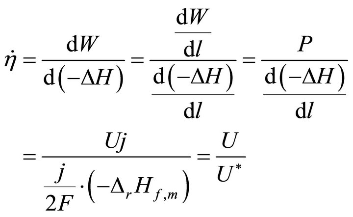
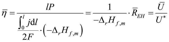
When W and ΔH tend towards infinitesimal, Formula (1) reflects the instantaneous efficiency of the ideal cell at one certain operating point and turns into Formula (2). In Formulae (2) and (3),  is the instantaneous efficiency, F is the Faraday constant, ΔrHf,m is the molar enthalpy change of the cell reaction, and U* denotes the thermalequivalent electromotive force (TEEF), a constant independent of temperature and pressure. For lower and higher heating value cells, TEEF is separately 1.282 V and 1.481 V as suggested by pioneering documents [1,7, 8]. These are the values under standard conditions.
 (2)
(2)
 (3)
(3)
From Formula (2) it can be seen that the instantaneous efficiency depends only on the voltage of the operating points. Such a simple dependence may mostly originate from the assumption that TEEF keeps constant. The assumption overlooks the little and changeful influence of minor factors and simplifies efficiency calculation, and it seems highly beneficial to the derivation of the average efficiency equation. In essence, the assumption may be double. It is known the molar enthalpy change of the cell reaction varies with operating temperature and species concentrations (or partial pressures). However, both variations may be so little in comparison with the Faraday constant under realistic operating conditions that they can be neglected and TEEF appears almost independent of operating temperature and species concentrations.
Formula (2) can be seen in or derived from public documents [1,7,8] as typical of the most concise form. Here it is termed the instantaneous efficiency equation and keeps valid only in the working zone of the ideal cell. The equation may represent a volt-ampere method to calculate the instantaneous efficiency with which no other variables need to be known than cell voltage (and current). Complex versions of the instantaneous efficiency formula can also be found in public documents [3,5], and they may represent non-volt-ampere methods with which current density and fuel consumption or supply need to be known besides voltage (and current). In the non-volt-ampere methods, addition energy or fuel consumptions are included in the chemical energy, as one of the ideologies and methodologies to deal with the efficiency problem. By consideration of the additional consumptions, the energy efficiency may be conceptually revised, and by measurement of fuel consumption or supply, the non-volt-ampere methods may be highly sensitive to measurement errors at small loads. Moreover, the complex expressions of the instantaneous efficiency with the non-volt-ampere methods may make it difficult or impossible to get the average efficiency expressed concisely and analytically.
2.3. Average Efficiency Equation
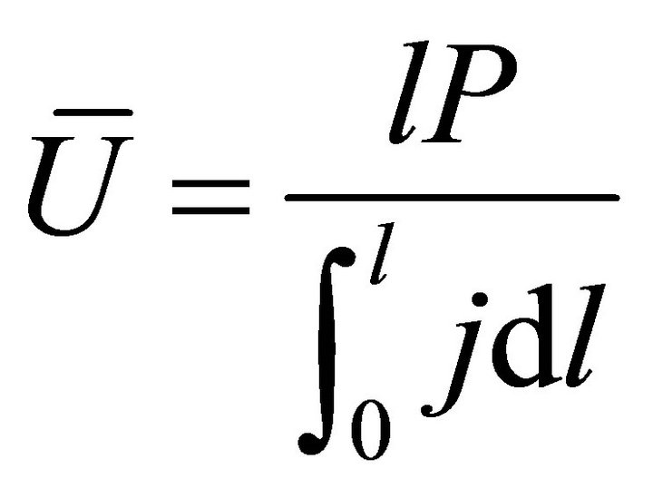
When W and ΔH are not infinitesimal, Formula (1) reflects the average efficiency of the ideal cell over a period of time. Under a fixed load P, the average efficiency during operating time l may be represented with Formula (4). In Formulae (4)-(6), ![]() ,
,  , and
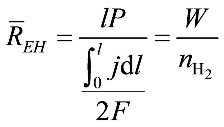
, and  are the average efficiency, the average electricity-hydrogen ratio, and the average voltage of the cell under load P, respectively, and
  denotes the number of moles of hydrogen consumed by the cell.
 (4)
(4)
 (5)
(5)
 (6)
(6)
It is seen from Formula (4) that the average efficiency is directly proportional to the average electricity-hydrogen ratio, and such a relationship also exists between the instantaneous efficiency and electricity-hydrogen ratio. Thus, the efficiency is in fact also the effective utilization index of fuel. It is also seen from Formula (4) that the average efficiency is directly proportional to the average voltage, which means that the average efficiency can be expressed formally as the instantaneous efficiency can.
Formula (4) may be difficult to use directly. In order to render it direct, the relationship between l and j should first be established. The relationship is determined jointly by the load and cell characteristic equations, as separately given in Formulae (7) and (8). The load characteristic equation represents the operating regime of the ideal cell, the constant-power mode; for real cells, this regime might be understood as the time-averaged one as well. The cell characteristic equation may approximately describe the volt-ampere movement of the ideal cell with time. Although this equation doesn’t hold in the activation polarization region, the derived average efficiency equation can approximately apply. See Section 3.2 for details.
 (7)
(7)
 (8)
(8)
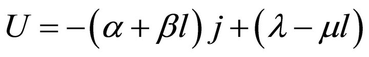
In Formula (8), α, β, λ and μ are all cell constants. α
and λ both are called the polarization constants, and they are separately the slope and intercept of the linear part of the initial steady-state polarization (SSP) curve. β and μ both are called the degradation constants, and they are separately the rates of change with time of α and λ. In the ideal cell model, there also exists the fifth cell constant, La, and it is the absolute lifetime of the cell.
Formulae (7) and (8) may define the l-j relationship. Substituting j for l according to the relationship in Formula (4) or (6) gives three expressions of the average efficiency during operating time l under load P, as given in Formulae (9)-(11), depending on three different kinds of cell degradation characteristics.
when  and
and ,
,
 (9)
(9)
when 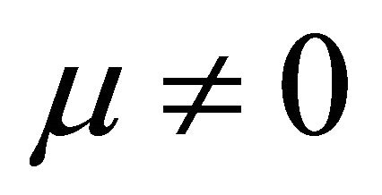 and
and ,
,
 (10)
(10)
when  and
and In Formulae (9)-(11), j0 is the initial current density of the cell under load P, which may be expressed as:
 (12)
(12)
Formulae (9)-(11) are just the analytical expressions of the average efficiency. All of them are called the average efficiency equation of PEM fuel cells, and they are all restricted by the boundaries of the working zone. Formulae (9)-(11) stand for the first form of the average efficiency equation, and the second form will be given in Section 3.1.
2.4. Generalization of Energy Efficiency Equations
The instantaneous efficiency equation, Formula (2), and the average efficiency equation, Formulae (9)-(11), may add up to a complete set of efficiency formulae of the ideal cell. These formulae may make sense only in the working zone of the cell.
 (11)
(11)
With the cell constants for cell specialty characterization, the average efficiency equation can be generalized to a diversity of real cells. The generalization can be performed through regularization of the degradation behavior of real cells. Once regularized, various real cells can be described formally like the ideal cell so that the average efficiency equation may approximately apply to real cells.
As for the instantaneous efficiency equation, its generality seems obvious, as it can be derived even free of the ideal cell model.
3. Overviews of Efficiency Evolutions
3.1. Transformation of the Average Efficiency Equation
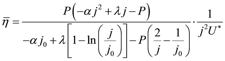
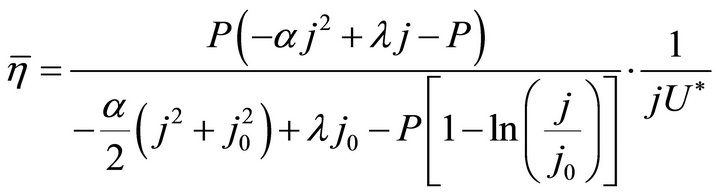
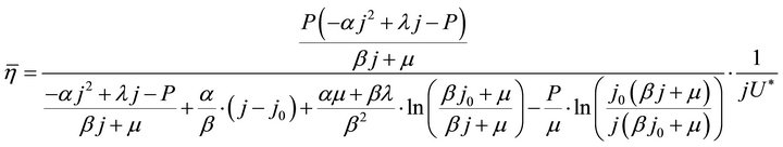
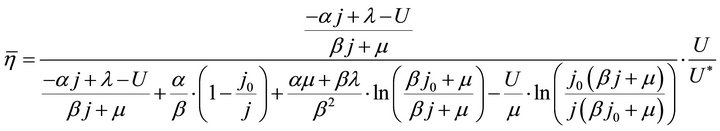
By substituting Formula (7) into Formulae (9)-(11), the second form of the average efficiency equation can be obtained, as represented by Formulae (13)-(15). These formulae may represent a simple method to calculate or predict the average efficiency only with the operating endpoint and cell constants, and besides, they may facilitate overviews of the evolutions of average efficiency. In them, j0 is given as Formula (16).
when  and
and ,
,
 (13)
(13)
when  and
and ,
,
 (14)
(14)
when  and
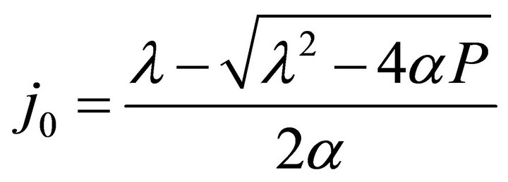
and where,
 (16)
(16)
It is known from Formulae (13)-(16), although the average efficiency essentially reflects the average process property of the cell over a period of time, it can be expressed with the individual state property of the corresponding operating endpoint. In this sense, the average efficiency of the cell over a period of time might be reliably referred to as the average efficiency of the operating end-point. It may be clearly seen, the average efficiency is the product of the instantaneous efficiency and a coefficient. The coefficient is also a state function involving cell constants.
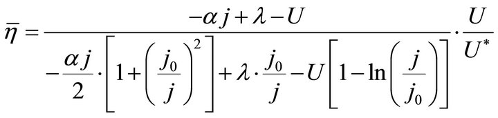
It is also known from Formulae (9)-(11) or (13)-(15) that the average efficiency evolutions may strongly depend on cell degradation characteristics. Although both β and μ can influence the average efficiency evolutions, but they don’t always appear in the efficiency equation. If both of them are not equal to 0, then both are included in the equation. If either of them is 0, then neither of them is included. For the two degradation characteristics,  and
and  and
and  and
and , though neither β nor μ appears in the equation, the dependences of the average efficiency on j, P, α, and λ are different.
3.2. Construction of Efficiency Distributions
For ideal and real cells, the instantaneous and average efficiencies may keep evolving with load magnitude and operating time. As known from Section 2, both of the instantaneous and average efficiencies can behave as one of the state functions of the cells, which means the evolutions can be turned into those with the operating point. In this way, the two single evolutions (as load magnitude and operating time) of both the instantaneous and average efficiencies can be outlined together in the working zone to give the instantaneous and average efficiency distributions.
As the instantaneous efficiency is directly proportional to the voltage, the operating points of the same voltage would constitute one line of equal instantaneous efficiency. Drawing such lines all over the working zone of one cell at regular intervals gives the instantaneous efficiency distribution of the cell. The average efficiency is not directly proportional to operating voltage, but Formulae (13)-(15) may be viewed as the average efficiency contour equation. Extend the Formulae to cover the nonlinear polarization region and draw the average efficiency contours at regular intervals in the working zone, then the average efficiency distribution can be obtained.
Deconvolution of the working zone may help analyze efficiency distributions and obverse efficiency evolutions. In one hand, the working zone may result from the sweep of SSP curve with operating time, so the evolution at one moment as load magnitude can be observed along the SSP curve at the moment. On the other hand, the work-
 (15)
(15)
ing zone may be viewed as composed of countless load curves, so the evolution at one load magnitude as operating time can be observed along the load curve. Besides, more other composite evolutions than the two single evolutions may also be overviewed from the distributions.
3.3. Examples of Efficiency Evolutions
The instantaneous and average efficiency distributions of three ideal cells of lower heating value are displayed in Figures 1 and 2 for overviews of the efficiency evolutions of the cells throughout their entire absolute lifetimes. Belonging to three different kinds of degradation characteristics, these cells are of the same polarization constants, long and different lifetimes and closely related degradation constants, as listed in Table 1. Long life-
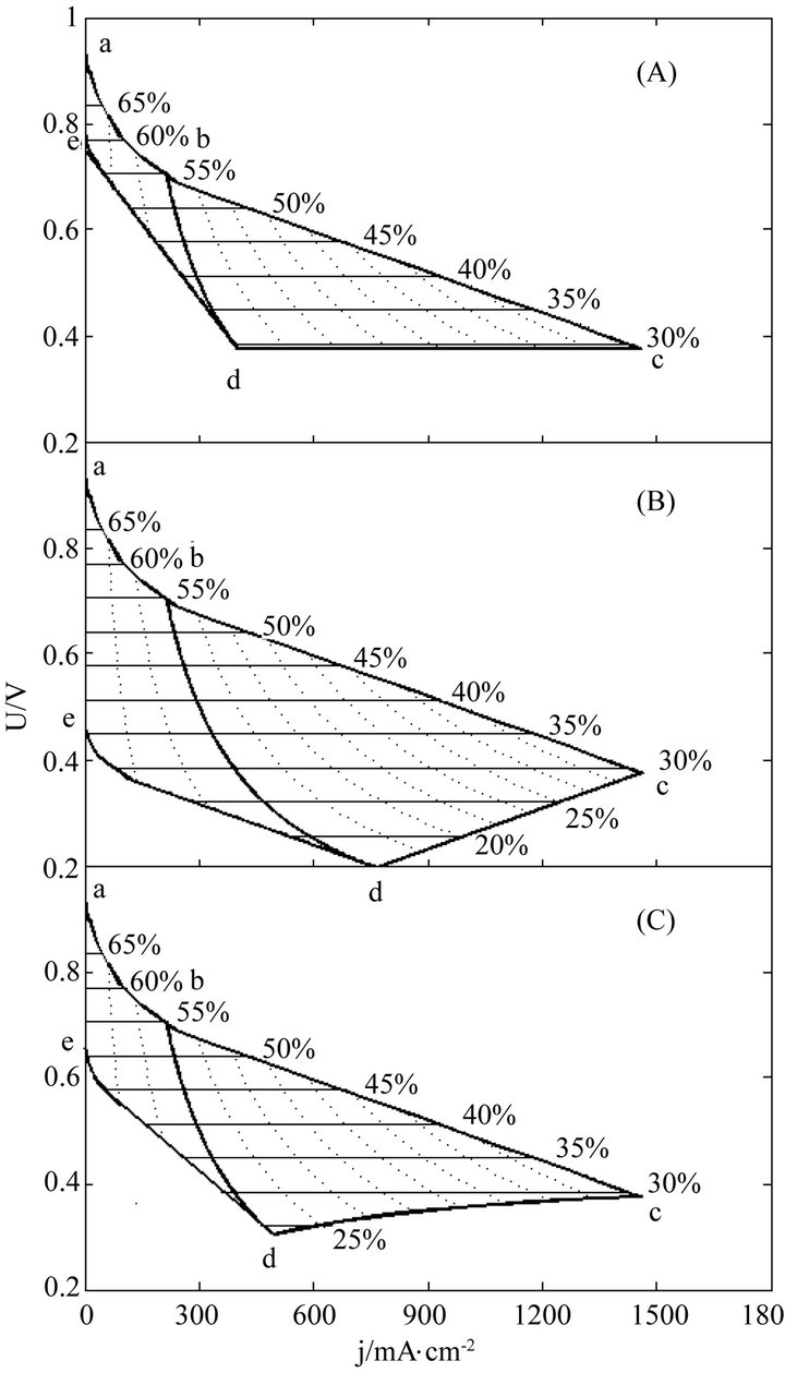
Figure 1. The instantaneous efficiency distributions of three ideal cells in their working zones under degradation characteristics of (A) μ = 0 and β ≠ 0; (B) μ ≠ 0 and β = 0 and (C) μ ≠ 0 and β ≠ 0. The critical load power density is 150 mW∙cm−2 and the load curves are at intervals of 50 mW∙cm−2 for each cell.
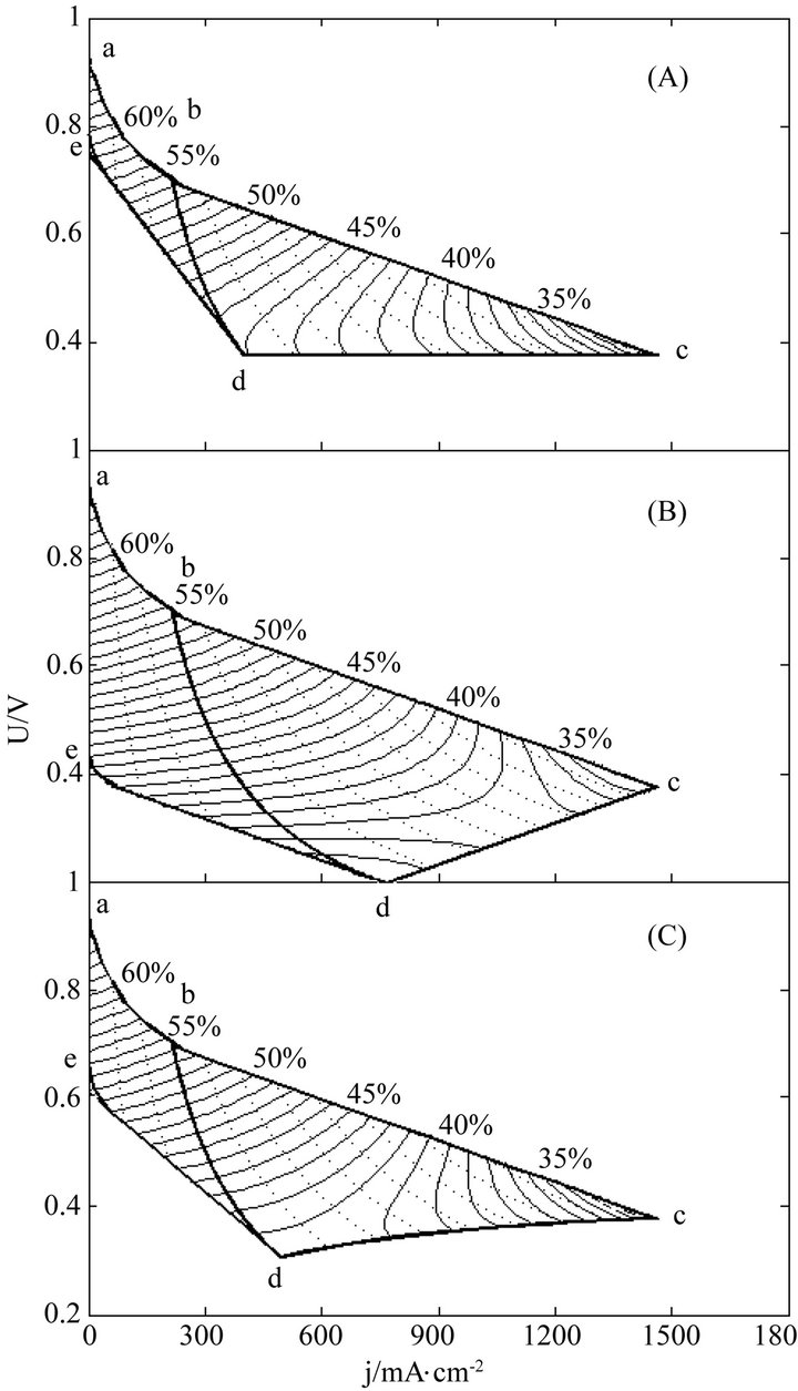
Figure 2. The average efficiency distributions of three ideal cells in their working zones under degradation characteristics of (A) μ = 0 and β ≠ 0; (B) μ ≠ 0 and β = 0 and (C) μ ≠ 0 and β ≠ 0. The critical load power density is 150 mW∙cm−2 and the load curves are at intervals of 50 mW∙cm−2 for each cell.
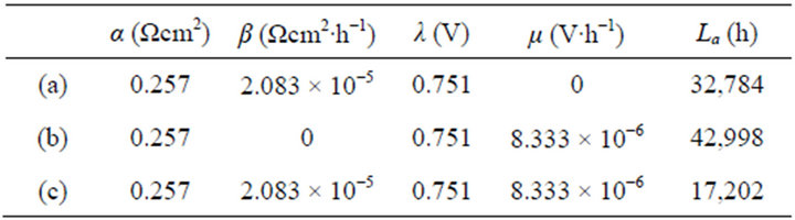
Table 1. The cell constant values in Figures 1 and 2.
times mean big working zones and wide visual fields. To see the efficiency evolutions at shortened lifetimes, just move the final SSP curve in and reduce the working zones, and the resultant efficiency evolution profiles are part of the original ones.
Once regularized, real cells may formally possess the just same properties and have the same efficiency evolution rules with ideal cells. This may greatly facilitate overall surveys of the efficiency evolutions of real cells. Figures 3-5 show three examples separately corresponding to two single cells and a 135-cell stack. They all are real samples of higher heating value and their working zones are all of ideally revised version [10]. As known from Table 2, they belong to three different kinds of degradation characteristics and have no close relationship in cell constant values. See documents [10-12] for details of these samples and see our recent work [10] for details of regularizations.
In these distributions, curves abc, de, cd and bd are the initial SSP curve, the final SSP curve (or the absolute lifetime end-curve), the relative lifetime end-curve and the critical load curve, respectively; points a and e separately are the starting points of the initial and final SSP curves; points c and d separately are the intersection points of the initial and final SSP curves with the relative lifetime end-curve; point b is the intersection point of the critical load curve with the initial SSP curve; and dotted load curves at regular intervals of power density are also given.
4. Discussion
4.1. The Role of Cell Constants
The energy efficiency formulae may greatly facilitate the estimation of the operating efficiency of PEM fuel cells,
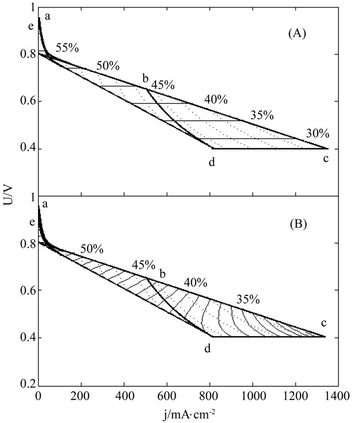
Figure 3. The (A) instantaneous and (B) average efficiency distributions of a real single cell of degradation characteristic of μ = 0 and β ≠ 0 in its ideally revised working zone. The critical load power density is 329 mW∙cm−2 and the load curves are at intervals of 50 mW∙cm−2.

Figure 4. The (A) instantaneous and (B) average efficiency distributions of another real single cell of degradation characteristic of μ ≠ 0 and β = 0 in its ideally revised working zone. The critical load power density is 492 mW∙cm−2 and the load curves are at intervals of 50 mW∙cm−2.
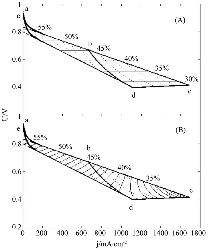
Figure 5. The (A) instantaneous and (B) average efficiency distributions of a real 150-cell stack of degradation characteristic of μ ≠ 0 and β ≠ 0 in its ideally revised working zone. The critical load power density is 449 mW∙cm−2 and the load curves are at intervals of 50 mW∙cm−2. U denotes unit-cell-averaged voltage.
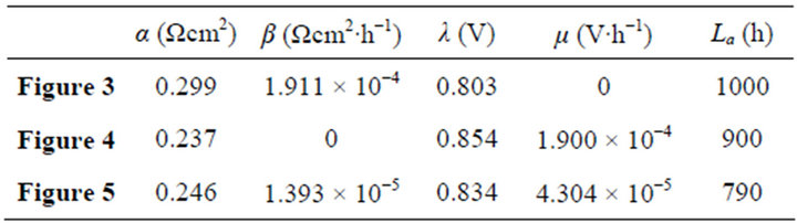
Table 2. The cell constant values in Figures 3-5.
as it seems almost unpractical to calculate the operating efficiency point by point throughout the operating range of the cells with the non-volt-ampere methods. In an extensive meaning, they might proximately apply to all types of fuel cells.
Two general trends may be seen from Figures 1 and 2 the efficiencies decrease with load magnitude and operating time, which may be ascribed to and reflect the polarization loss and degradation loss. The instantaneous efficiency evolutions are simple, while the average efficiency evolutions are complex. The complexity may come from the internal combined contributions of three major factors including cell performance, degradation and service life time, and the average efficiency formulae may well describe the complexity.
The energy efficiency formulae may be understood as the concise and inclusive representations of the compositive influence of the related factors on the energy efficiency. In the formulae, the cell constants may function as the resultant and intermediary parameters to correlate the related factors with the average efficiency. The related factors include component properties, production methods, operating conditions, and so on, thus one can estimate their influence on the efficiency through estimation of their impacts on cell constants.
4.2. Errors and Reduction
4.2.1. From Formula Coverage Extension
It can be seen from Figure 2, although Formula (8) doesn’t hold in the activation polarization part of the working zones, the resultant evolution profiles of the average efficiency in the part appear logical, which may mean the average efficiency equation, Formulae (13)- (15), approximately applies to the part as well. The treatment of the activation polarization part was not involved in the ideal cell model, thus the extension of the average efficiency equation to cover this part appears a supplement.
The initial SSP curve defined by Formula (8) can be regarded as an auxiliary line to divide the part into two plots, and with the auxiliary line as the suppositional initial SSP line for both plots, the average efficiency can be evaluated everywhere in the part. Because of the virtual time applied in both plots, the treatment leads to a slight underestimation of the average efficiency in the part, and the efficiency data should be read in company with the crude SSP curves and load curves in the part. Actually, the average efficiency equation is derived without consideration of time, and it gets the entire profiles one-time drawn.
For quite a few real cells, the extension of the formulae coverage seems unnecessary because the activation polarization part seems so small that it can be disregarded. Figures 3-5 are just of such samples.
4.2.2. From Cell Regularization
The general evolution trends may still exist in real cells as seen from Figures 3-5. Obviously, the trends originate from the adaptions of real cells to ideal cells. The adaption may produce some calculation error as well, as one of the negative consequences of the use of cell constants. However, with respect to error reduction, the regularization might make this method more attractive than the non-volt-ampere methods, especially in the range of small current density.
The load-dependent evolution trend of the instantaneous efficiency displayed in Figures 3-5 appears different from what have been given in some of previous documents [4-6]. In them were the evolution profiles with a maximum instantaneous efficiency, i.e. the instantaneous efficiency increases with current density in certain ranges of low current density. Such abnormal profiles may be of the non-volt-ampere methods [3,5,9], but under small loads calculation errors may be not ignored either. With the non-volt-ampere methods, any small measurement error in fuel consumption or fuel supply may incur a great calculation error in the instantaneous efficiency under small loads. For this reason and more in consideration of the straitness of the error-sensitive ranges, prudential practices [1,3,6] may be to give no examination of the efficiency in a narrow current range adjacent to open circuit voltage.
4.2.3. From Constant-TEEF Assumption
One more problem that is worth further discussion on the formulization of the energy efficiency may be the use of the TEEF constant. This refers to the different TEEF constant values taken for the lower and higher heating value cells. When cells operate at the temperatures near the boiling point of water, it may be difficult to determine which value is taken for the calculation, and whichever is chosen, an error may be unavoidable. Such an error may be attributed to the implication of the chemical energy. When phase change is involved in the energy conversion, whether phase change heat counts toward the chemical energy may affect calculation result. This may be a matter of theory as it needs to be made clear whether or not liquid water is the direct product of the electrochemical reaction below the boiling point. In the current measure, to reduce error, interpolation method may be considered for TEEF constant determination near the boiling point of water.
4.3. On Efficiency Comparison
Acquaintance with the general trends and vast panoramas of the efficiency evolutions of ideal and real cells may bring up the subject of rational efficiency comparison and make a basic contradiction between efficient and full uses of cells emerge. For a rational comparison, great emphasis may be placed on average efficiency instead of instantaneous efficiency, so that the focus may shift on to selection of operating end-point for each of involved cells and a basic contradiction between efficient and full uses of cells comes out. On balance, the average energy efficiency may be cumbered with the average power generation cost. Overuse may lead to low efficiency and high efficiency may go against full use. At last, the resolution of the contradiction may turn to the maximization of cost performance.
5. Conclusions
The energy efficiency movements of PEM fuel cells with load and time are uniformly described with the volt- ampere method for a diversity of real cells and the energy efficiency evolutions are well displayed over the working zones of the cells. The main conclusions include:
1) By neglecting the changeful and minor of the influence of operating temperature and species concentrations, the instantaneous and average efficiency movements can be concisely and adequately described separately with one and three formulae based on the five-constant idea cell model.
2) The instantaneous efficiency only depends on and is in direct proportion to operating voltage. The average efficiency has no simple loadand time-dependences unlike the instantaneous efficiency, but it can also be analytically expressed in the form of the state function of operating end-point like the instantaneous efficiency.
3) The average efficiency closely depends on degradation characteristics among others. However, although both degradation constants affect the average efficiency, but they don’t always appear in the formulae. If both of them are not equal to 0, then both are included in the equation. If either of them is 0, then neither of them is included.
4) The efficiency formulae can be translated to a diversity of real cells by formal revision of them. With the formulae, both the loadand time-dependent movements of both the instantaneous and average efficiencies can be overviewed throughout the whole working zone of the cells in the form of energy efficiency distribution.
5) Ascribed to and reflecting the polarization loss and degradation loss, the general trends are exhibited both the instantaneous and average efficiencies decrease with load magnitude and operating time throughout the working zones of ideal and real cells.
6. Acknowledgements
This work has been supported by the National 973 Program (No. 2012CB215500), the National 863 Programs (No. 2012AA053402, No. 2012AA053 402) and the Specialized Research Fund for the Doctoral Program of Higher Education (No. 20090002110074) of China.
REFERENCES
- F. Barbir and G. Gómez, “Efficiency and Economics of Proton Exchange Membrane (PEM) Fuel Cells,” International Journal of Hydrogen Energy, Vol. 22, No. 10-11, 1997, pp. 1027-1037. doi:10.1016/S0360-3199(96)00175-9
- A. Kazim, “A Novel Approach on the Determination of the Minimal Operating Efficiency of a PEM Fuel Cell,” Renewable Energy, Vol. 26, No. 2-3, 2002, pp. 479-488. doi:10.1016/S0960-1481(01)00083-0
- A. E. Gonnet, S. Robles and L. Moro, “Performance Study of a PEM Fuel Cell,” International Journal of Hydrogen Energy, Vol. 37, No. 19, 2012, pp. 14757-14760. doi:10.1016/j.ijhydene.2011.12.076
- X. Zhang, J. Guo and J. Chen, “The Parametric Optimum Analysis of a Proton Exchange Membrane (PEM) Fuel Cell and Its Load Matching,” Energy, Vol. 35, No. 12, 2010, pp. 5294-5299. doi:10.1016/j.energy.2010.07.034
- J. I. San Martin, I. Zamora, J. J. San Martin, V. Aperribay, E. Torres and P. Eguia, “Influence of the Rated Power in the Performance of Different Proton Exchange Membrane (PEM) Fuel Cells,” Energy, Vol. 35, No. 5, 2010, pp. 1898-1907. doi:10.1016/j.energy.2009.12.038
- Y. Hou, B. Wang and Z. Yang, “A Method for Evaluating the Efficiency of PEM Fuel Cell Engine,” Applied Energy, Vol. 88, No. 4, 2011, pp. 1181-1186. doi:10.1016/j.apenergy.2010.10.040
- C. S. Spiegel, “Designing & Building Fuel Cells,” Simplified Chinese Translation Edition, McGraw-Hill Education (Asia) Co. and Publishing House of Electronics Industry, Beijing, 2008.
- J. Larminie and A. Dicks, “Fuel Cell Systems Explained,” John Wiley & Sons Ltd, Chichester, 2000.
- S. H. Seo and C. S. Lee, “A Study on the Overall Efficiency of Direct Methanol Fuel Cell by Methanol Crossover Current,” Applied Energy, Vol. 87, No. 8, pp. 2597- 2604. doi:10.1016/j.apenergy.2010.01.018
- H. F. Zhang, P. C. Pei, X. Yuan and X. Z. Wang, “Regularization of the Degradation Behavior and Working Zone of Proton Exchange Membrane Fuel Cells with a Five-Constant Ideal Cell as Prototype,” Energy Conversion and Management, Vol. 52, No. 10, 2011, pp. 3189- 3196. doi:10.1016/j.enconman.2011.04.022
- D. Liu and S. Case, “Durability Study of Proton Exchange Membrane Fuel Cells under Dynamic Testing Conditions with Cyclic Current Profile,” Journal of Power Sources, Vol. 162, No. 1, 2006, pp. 521-531. doi:10.1016/j.jpowsour.2006.07.007
- M. Prasanna, E. A. Cho, T. H. Lim and I. H. Oh, “Effects of MEA Fabrication Method on Durability of Polymer Electrolyte Membrane Fuel Cells,” Electrochimica Acta, Vol. 53, No. 16, 2008, pp. 5434-5441. doi:10.1016/j.electacta.2008.02.068
NOTES
*Corresponding author.