Communications and Network
Vol.5 No.1(2013), Article ID:28236,16 pages DOI:10.4236/cn.2013.51004
Adaptive Routing Algorithms and Implementation for TESH Network
1Shonan Institute of Technology, Kanagawa, Japan
2ACS Co., Ltd., Tokyo, Japan
3International Islamic University Malaysia (IIUM), Kuala Lumpur, Malaysia
Email: miu@info.shonan-it.ac.jp, m-kaneko@acs21.co.jp, rahmanjaist@gmail.com, watanabe@info.shonan-it.ac.jp
Received October 30, 2012; revised December 1, 2012; accepted January 2, 2013
Keywords: TESH Network; Adaptive Routing Algorithm; Hardware Cost; Router Delay; Communication Performance
ABSTRACT
The Tori-connected mESH (TESH) Network is a k-ary n-cube networks of multiple basic modules, in which the basic modules are 2D-mesh networks that are hierarchically interconnected for higher level k-ary n-cube networks. Many adaptive routing algorithms for k-ary n-cube networks have already been proposed. Thus, those algorithms can also be applied to TESH network. We have proposed three adaptive routing algorithms—channel-selection, link-selection, and dynamic dimension reversal—for the efficient use of network resources of a TESH network to improve dynamic communication performance. In this paper, we implement these routers using VHDL and evaluate the hardware cost and delay for the proposed routing algorithms and compare it with the dimension order routing. The delay and hardware cost of the proposed adaptive routing algorithms are almost equal to that and slightly higher than that of dimension order routing, respectively. Also we evaluate the communication performance with hardware implementation. It is found that the communication performance of a TESH network using these adaptive algorithms is better than when the dimension-order routing algorithm is used.
1. Introduction
Interconnection networks are the key elements for building massively parallel computers consisting of hundreds or thousands of processors [1]. Recent progress in verylarge-scale integration (VLSI) and network-on-chip (NoC) technology has led to multicomputer systems on threedimensional LSIs. A Tori connected mESH (TESH) network [2-6] is a hierarchical interconnection network for large-scale on-chip multicomputers. It consists of multiple basic modules (BMs) which are 2D-mesh networks and the BMs are hierarchically interconnected by a 2Dtorus (k-ary 2-cube) to build higher level networks. Restricted use of physical links between silicon planes reduced performance of the TESH network.
We have proposed a deterministic, dimension-order routing algorithm [7] for the TESH network and have shown that Level-3 TESH networks have higher performance than a k-ary 2-cube. The minimum number of virtual channels per link in dimension order routing has been proven to be two. Thus, additional virtual channels can improve communication performance such as packet transfer time and network throughput. An adaptive routing algorithm can also be implemented using additional virtual channels [8].
Many adaptive routing algorithms have been proposed for k-ary n-cube networks [9-13]. Based on these algorithms, we have proposed three adaptive routing algorithms for TESH [14,15]. In [14], three adaptive routing algorithms were proposed. However, the performance is evaluated using computer simulation only. Obviously, it is necessary to evaluate the router delay with practical hardware implementation of the proposed routing algorithms. In [15], two selection algorithms are implemented in hardware and their hardware cost is compared with the dimension order router. However, the dynamic dimension reversal routing is not implemented in [15]. Router delay with hardware implementation of any of these algorithms is not studied yet. The main objective of this paper is the hardware implementation of the proposed adaptive routing algorithms of TESH network.
The remainder of the paper is organized as follows. In Section 2, we briefly describe the basic structure of the TESH network. The deterministic dimension-order routing is presented in Section 3 and the proposed adaptive routing algorithms are presented in Section 4. Hardware implementation and performance evaluation are discussed in Sections 5 and 6, respectively. Finally, Section 7 presents the conclusion.
2. Interconnection of the TESH Network
The Tori-connected mESH (TESH) Network is a hierarchical interconnection network consisting of Basic Modules (BM) that are hierarchically interconnected to form a higher level network. The BM of the TESH network is a 2D-mesh network of size . In this paper, unless specified otherwise, BM refers to a Level-1 network. Successively higher level networks are built by recursively interconnecting immediately lower level subnetworks in a 2D-torus network. A higher-level network is built using immediate lower level networks as subnet modules as a 2D-torus network of size
  [2]. Here m is a positive integer and in this paper, we have considered m=2 i.e.,
  2D-mesh as BMs and
  2D-torus (k-ary 2-cube) as higher level networks as shown in Figure 1.
A  BM has
  free ports at the contours for higher level interconnection. For each higher level interconnection, a BM uses
  of its free links,
  free links for vertical interconnections and
  free links for horizontal interconnections. Here,
  is the inter-level connectivity.
  leads to minimal inter-level connectivity, while
  leads to maximum inter-level connectivity. Considering the size of the basic module m, level of hierarchy n, and inter-level connectivity q, we can define the TESH network as
  networks. Since we have considered
 , a Level-2 network, can be formed by interconnecting
  BMs. Similarly, a Level-3 network can be formed by interconnecting 1 Level-2 subnetworks, and so on. Each BM is connected to its logically adjacent BMs. To avoid clutter, the wraparound links of the BMs are not shown in Figure 1. In the rest of this paper we consider
 , therefore, we focus on a class of
  networks.
The highest level network which can be built from  BM is
BM is . With
  and
and ,
,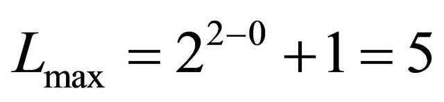 . The total number of nodes in a TESH network is
 . Using maximum level of hierarchy,
  , the maximum number of nodes which can be interconnected by a
is . With
  a Level-2 TESH network consists of 256 nodes. Similarly a Level-3 networks consists of 4096 nodes.
Processing elements (PEs) or node in a  network are addressed using base-
 numbers as follows.
 (1)
(1)
Here,  is the location of a subnetwork at level i-1. For example, in a Level-3 TESH with
 , each PE is addressed by a base-4 number n = n5n4n3n2n1n0, where
  and
and  address of a PE in the Level-3 network,
  and
and  address of a PE in the Level-2 network, and
  and
and  address of a PE in the BM. The numerical values shown in Figure 1 are at BM address
 ![]() of a Level-2 TESH network.
of a Level-2 TESH network.
The assignment of free ports for inter-level connections for the higher level networks has been done quite carefully so as to minimize the higher level traffic through the BM. The address of a node  encompasses in
  is represented as
 . The address of a node
  encompasses in
  is represented as
 . The node
  in
in  and
and  in
in  are connected by a link if the following condition is satisfied.
 (2)
(2)
where .
.
It is shown in Figure 1 that for a Level-2 TESH network,  connects with either
  or
or  in the x-direction, i.e.,
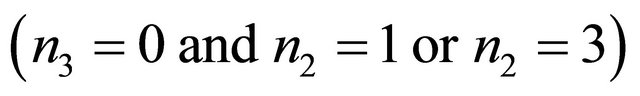 and with either BM(1,0) or BM(3,0) in the y-direction, i.e.,
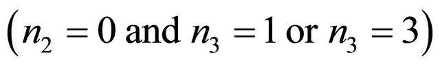 .
.
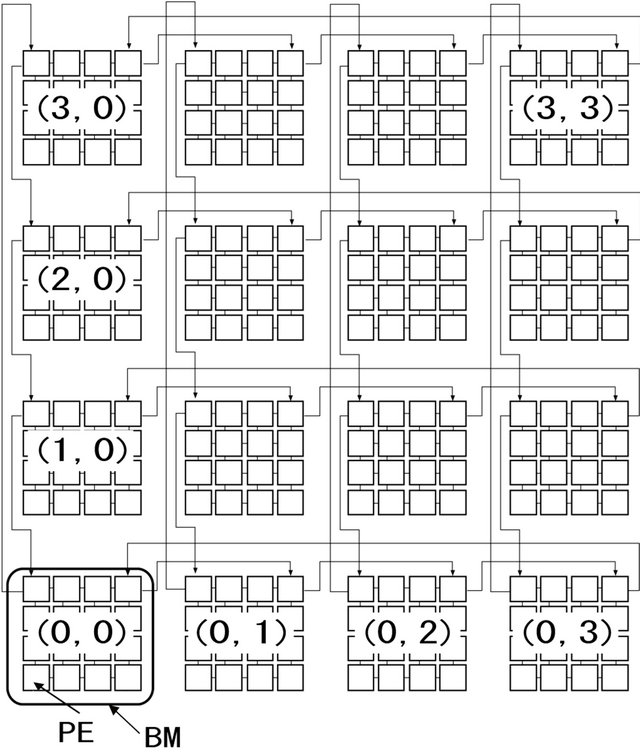
Figure 1. Hierarchical interconnection of Level-2 TESH network.
3. Dimension-Order Routing
A routing algorithm determines the path a packet takes as it travels through the network from its source to destination. A deterministic, dimension-order routing for a TESH network [7] transfers packets from higher-levels to lower-levels. That is, it is first done at the highest level network; then, after the packet reaches its highest level sub-destination, routing continues within the subnetwork to the next lower level sub-destination. This process is repeated until the packet arrives at its final destination. Packets passing through inter-BM links are forwarded from a vertical link to a horizontal link at the same level. When they arrive at the destination BM, they are transferred to the destination PE. The deterministic, dimension-order routing of Level-L TESH networks can generally be classified into the following three phases [7].
Phase 1: Intra-BM transfer path from source node to the outlet PE of the BM. (PEs which hold  or
or )
)
Phase 2: Higher level transfer path.
Phase 3: Intra-BM transfer path from the outlet of the inter-BM transfer path to the destination PE.
Phase 2 is divided into the following sub-phases:
Sub-phase 2.i.1: Intra-BM transfer to the outlet PE of Level  through the y-link/vertical link.
Sub-phase 2.i.2: Inter-BM transfer of Level  through the y-link/vertical link.
Sub-phase 2.i.3: Intra-BM transfer to the outlet PE of Level  through the $x$-link/horizontal link.
Sub-phase 2.i.4: Inter-BM transfer of Level  through the x-link/horizontal link.
Here, .
.
We have considered the dimension order routing algorithm for the TESH network. We use the following strategy: at each level, vertical routing is performed first. Once the packet reaches the correct row, then horizontal routing is performed. Routing in the TESH network is strictly defined by the source node address and the destination node address. Let a source node address be  and a destination node address be
 . The dimension-order of the TESH network is represented by
 . Figure 2 shows the routing algorithm
  for the TESH network, and Figure 3 shows the flow chart of it. The function get_group_number is the function to get group number. Arguments of this function are source PE address
 ![]() destination PE address
destination PE address![]() , and direction. The function
, and direction. The function  and
and  are the function to get the value
  of
of ![]() coordinate and
coordinate and  of y coordinate of a PE n that has an inter-BM link. Variables
  are group
  $g, level
 , dimension
 , and direction
 , respectively [7].
4. Adaptive Routing Algorithm
Adaptive routing algorithms for TESH networks are classified into two groups: local and global algorithms. Local algorithms are defined as adaptive routing algorithms that run in one phase and global algorithms are defined as algorithms for which the order of phases can be changed.
In this section, we introduce two local adaptive routing algorithms called as channel select (CS) and link select (LS); and one global adaptive routing algorithm called dynamic dimension reversal (DDR) [14].
The deadlock in a k-ary n-cube network can be avoided using 2 virtual channels using following two conditions [11].
Condition 1: Initially, first virtual channel (Channel-L) is used.
Condition 2: Then the packet move to the second virtual channel (Channel-H) if the wraparound links is used for routing.
Local algorithms for TESH network are applied in sub-phases 2.i.2 or 2.i.4 in Section 3. Because a ring network is formed using 4 outlet PEs (m = 2) and inter-BM links. Local adaptive routing algorithms can be applied in this ring of TESH network. To discuss local adaptive routing algorithms, we allocate a local PE address to each of those four PEs. Let ![]() be the local PE addresses of a ring network in the TESH. Then,
be the local PE addresses of a ring network in the TESH. Then, ![]() are addressed as follows:
are addressed as follows:
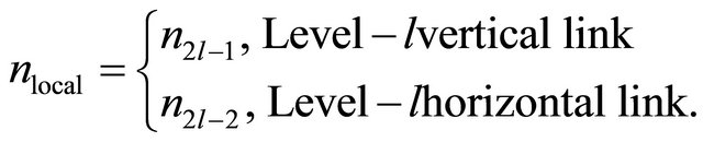 (3)
(3)
where ![]() and
and  are the PE address defined in section
 . Below, we discuss two local algorithms for a 4-PE ring network in TESH by using
![]() .
.
Since the higher-level links of TESH have k-ary n-cube network, adaptive routings of k-ary n-cube can be applied to TESH. Dynamic dimension reversal routing (DDR) [11] is proposed as adaptive routing algorithms of k-ary n-cube network. This algorithm has a lot of choice of the path and needs a few additional virtual channels. The DDR routing can also be applied to TESH network. However, unlike conventional k-ary n-cube network, the higher-level links are located in different PE in the TESH network. This is why, the choice of routing path in the TESH network is limited in comparison with k-ary ncube network.
4.1. Channel Select (CS) Algorithm
To avoid deadlock in a ring network, two virtual channels (Channel-L and Channel-H) are needed in each direction. The CS algorithm is an adaptive routing algorithm that can use those channels freely. When wraparound channels are not used in routing, for example in
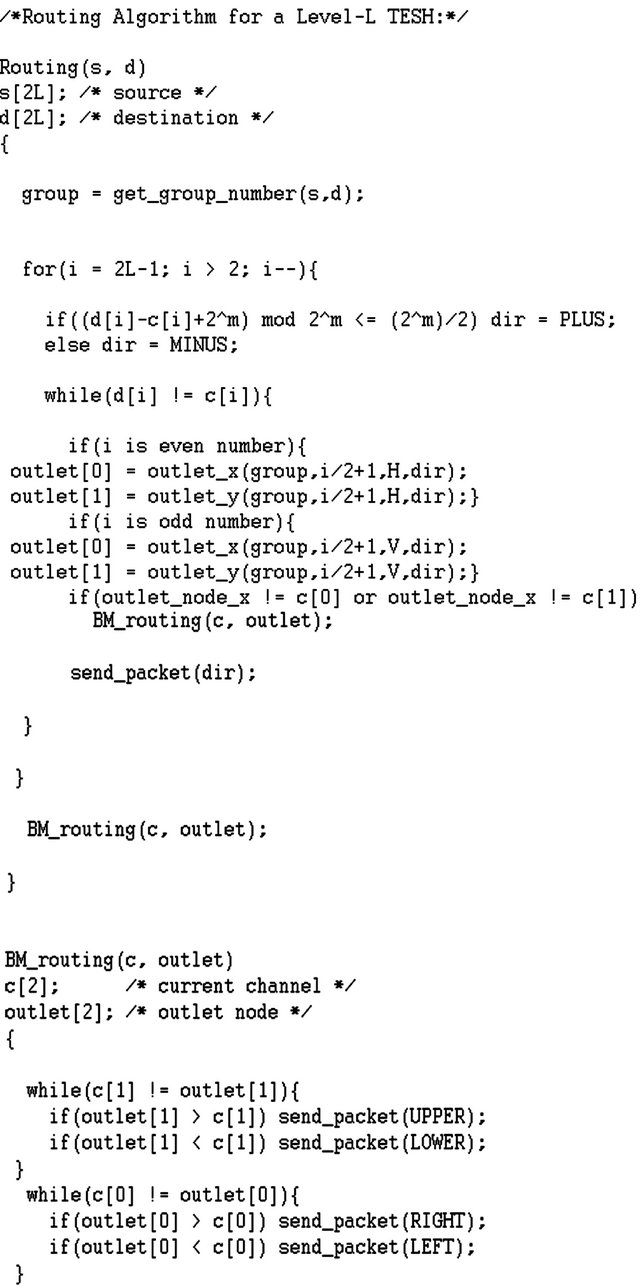
Figure 2. Routing algorithm of a TESH network.
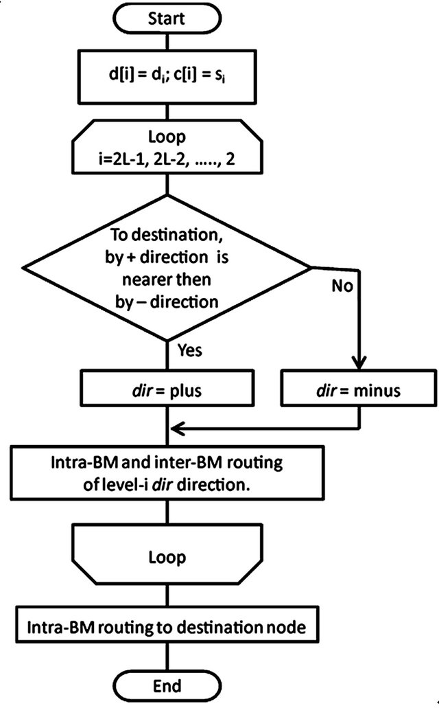
Figure 3. The flow chart of the dimension-order routing.
the routing from  to
to , only Channel-L is used. In this case, because ChannelH is not used in dimension-order routing, it is possible to move from Channel-L to Channel-H or use Channel-H initially. When the routing is terminated at the output PE of a wraparound channel such as the routing from
  to
to , only Channel-L is required. Therefore, it is possible to move from Channel-L to Channel-H or use Channel-H initially.
For dimension-order routing in a 4-PE ring network, the conditions for using only Channel-L are as follows:
Wraparound channels are not used in routing.
The routing is terminated at the output PE of a wraparound channel.
When the above conditions hold, the virtual channels are used according to the following order:
Either Channel-L or Channel-H is used.
The packet moves from Channel-L to Channel-H in the routing path.
The CS algorithm is an adaptive routing algorithm that can use virtual channels effectively. When the following three conditions hold in a 4-PE bidirectional ring network is deadlock-free [14]. The routing algorithm that applies this channel-selection principle is denoted as .
.
Condition-1: Use Channel-L initially.
Condition-2: Use Channel-H when a wrap-around link exists in the higher level network.
Condition-3: When a packet is in a Channel-L satisfies either of the following conditions, it can move to Channel-H.
Wrap-around links are not used in routing.
The routing will be terminated at the output PE of a wraparound link.
Theorem 1: Suppose the routing algorithm  of a TESH network is deadlock-free. The routing algorithm
  which apply CS algorithm in the inter-BM links of a TESH network is also deadlock-free.
Proof: The dimension-order routing of the TESH network  is deadlock-free [7]. Phase 1, phase 3, sub-phase 2.i.1, and sub-phase 2.i.3 are deadlock-free because those phases are used to route packet in the mesh network and remains exactly same as routing algorithm
 . Sub-phase 2.i.2 and 2.i.4 form a
  -PE ring network in each direction. According to Yang’s adaptive routing [9], the routing of packets in these sub-phases which applies CS algorithm is deadlock-free. Therefore, the proposed CS algorithm for the TESH network,
  , is deadlock free.
4.2. Link Select (LS) Algorithm
Sub-phases 2.i.2 and 2.i.4 form a ring network. If the number of hops from the source PE to the destination PE is equal in the clockwise direction and in the counter-clockwise direction, then the packet can follow either of these two directions. The distance from  to
to  in a 4-PE ring network is 2 in both the clockwise and counter-clockwise direction. Packet can follow path-a in the clockwise direction or path-b in the counter-clockwise direction.
If the following equation is satisfied, a packet can select from either a clockwise or counter-clockwise direction.
 (4)
(4)
where s and d denote the source and destination PE addresses, respectively. The routing algorithm that applies this link-selection principle is denoted as .
.
Theorem 2: Suppose routing algorithm  of the TESH network is deadlock-free. The routing algorithm
  which applies the LS algorithm to Inter-BM links of the TESH network is also deadlock-free.
Proof: The proposed LS algorithm enforces some routing restrictions as dimension order routing to make the routing algorithm simple and avoid deadlocks. Routing order of phases and sub-phases are strictly followed to route packet. If each phase is deadlock-free, then entire routing algorithm ensures the freedom from deadlock. Phase 1, phase 3, sub-phase 2.i.1, and sub-phase 2.i.3 are deadlock-free because those phases are used to route packet in the mesh network and remains exactly same as routing algorithm . The routing algorithm
  of a TESH network is deadlock-free [7]. The topology of network in sub-phase 2.i.2 and 2.i.4 is bi-directional ring network. Dimension-order routing in a ring network is deadlock free with 2 virtual channels [10]. Therefore, the proposed LS algorithm for the TESH network,
  , is deadlock free.
The CS algorithm is used to select a virtual channel in a physical link and the LS algorithm is used to select a physical link in a network. Therefore, both the CS and LS algorithms can be applied at the same time. The routing algorithm that applies both the CS and LS algorithms is denoted as .
.
4.3. Dynamic Dimension Reversal (DDR) Algorithm
The dimension-order routing strictly maintain the restriction of routing dimension in an interconnection network, such as k-ary n-cubes. In the dimension-order routing for the TESH network the order of routing phases is fixed. However, an algorithm that can break the dimension order has already been proposed [11]. In this paper, the Dimension Reversal (DR) routing algorithm is applied in the TESH network. Dimension reversal routings of k-ary n-cubes are classified into two types: Static Dimension Reversal and Dynamic Dimension Reversal. Because Dynamic Dimension Reversal routing (DDR) can use channels efficiently, we apply DDR to a TESH. We called it as global adaptive routing algorithm. The DDR algorithm can be applied individually and simultaneously with the CS and LS algorithms.
In the DDR algorithm, each packet has a DR number, which is a count of the number of times that a packet has been routed from a channel in sub-phase ![]() to a channel in a lower-order sub-phase
to a channel in a lower-order sub-phase , q < p. Here, the format of p and q are
  and
and . We assume that
  and
and  are the high-order digits and
  and
and  are the low-order digits when p and q are compared. DR numbers are assigned as follows:
1) All packets are initialized with a DR of 0.
2) If a a packet routes from a channel  of subphase
 ![]() to a channel
to a channel  of sub-phase
 , then its DR is incremented.
The DDR algorithm divides the virtual channels into two classes: adaptive and deterministic. Packets originate in the adaptive channels and while they are in adaptive channels, they may be routed by adaptive routing. Whenever a packet acquires a channel, it labels the channel with its DR number. To avoid deadlock, a packet with a DR of p need not to wait for a channel labeled with a DR of q if . A packet that reaches a node where all output channels are occupied by packets with equal or lower DR numbers must switch to the deterministic channels. When a packet enters the deterministic channels, it must be routed by dimensionorder routing and cannot re-enter the adaptive channels.
The adaptive routing algorithm for the adaptive channel is as follows. A packet with DDR routing of a k-ary n-cube network can be routed in any direction using adaptive channels. However, since a TESH is a hierarchical network, higher-level links of a $ k-ary n-cube network, where each node of this k-ary n-cube is not located in the same BM. Therefore, the packet cannot be routed freely.
There are four outlet PEs in an inter-BM links in each BM as shown in Figure 1. When the packet goes through those PEs during intra-BM routing, it can select a path from the following ones:
Path 1: Interrupt the intra-BM routing and select the inter-BM link.
Path 2: Continue the intra-BM routing.
When the above conditions hold, the packet selects path-1 first.
An example of the DDR algorithm applied to a TESH network is shown in Figure 4. The half-tone PE is the source PE, and the solid arrow in the BM is the deterministic routing path. In this example, we assume that a packet goes through first in a Level-3 vertical link and next in a Level-3 horizontal link. In the dimensionorder routing of a TESH network, a packet is forwarded to the outlet PE of a Level-3 vertical link in phase 1 routing. However, in the DDR routing as shown in Figure 4 the packet goes through the outlet PE of a Level-3 horizontal link. When the packet reaches the outlet PE, it checks whether the Level-3 horizontal link is available or not. If it is available, the packet selects Path-1 and uses the Level-3 horizontal link before going to the outlet PE of the Level-3 vertical link. If it is not available, the packet selects Path-2 and continues with the phase 1 transfer. The routing algorithm that applies this DDR principle is denoted as .
.
Theorem 3: Suppose routing algorithm  of a TESH network is deadlock-free. The routing algorithm
  which apply the DDR algorithm to routing algorithm
  is also deadlock-free.
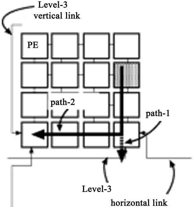
Figure 4. DDR algorithm in a TESH.
Proof: This theorem is proven by contradiction. If the network is deadlocked, then there is a set of packets P waiting for virtual channels held by other packets in P. There exists a packet that have maximum dimension reversal (DR) number , such that the DR of
 . Let
. Let  be the next channel selected for a packet with
 . From the condition of waiting for virtual channels in DDR algorithm,
 . This means that there are packets where
 . This is against a definition of
 . Therefore, the supposition that deadlock is occurred doesn't work out.
Let  be the next channel selected for a packet
 , and let r be the DR label of
 . Then
  where
where  is occupied by
 . However,
  is not permitted to wait on
  since
since . Because packet
  can go to deterministic channels. There is no deadlock in adaptive channels. Because the set of deterministic channels is deadlock-free, DDR algorithm
  of the TESH network is deadlock-free.
The CS, LS, and DDR algorithms applies in the different resources of a network, Thus, these algorithms can be applied simultaneously to a network. The routing algorithm that applies the CS, LS, and DDR algorithms simultaneously is denoted as R.
5. Hardware Implementation
5.1. Router Design
To evaluate the delay and hardware cost of our proposed algorithms, we designed an actual router using VHDL (very-high-speed integrated circuit hardware description language). The number of logic gates and the number of memory elements were evaluated using the tool from Xilinx Co. Ltd.
The entire circuit is shown in Figure 5. The circuit design was based on a general wormhole router [16] and the network-on-chip (NoC) technique [17,18] was used. In this evaluation, the number of links is 4 and the number of virtual channels in each link is 2. Because the amount of hardware used in a NoC is limited, the unconstrained use of buffers is prohibited. Thus, the number of buffers in each link is set to 4. The circuit of this routers control block is shown in Figure 6. The data flow of the control block consists of four pipelining stages: viz., link-channel selection (stage-1), arbitration (stage-2), buffer check (stage-3), and switching (stage-4). The link-selection and channel-selection circuits are included in stage-1. Their delays have a direct effect on the delay of the control circuit.
The increase in delay is caused by the complexity of the circuit for selection function that selects the next
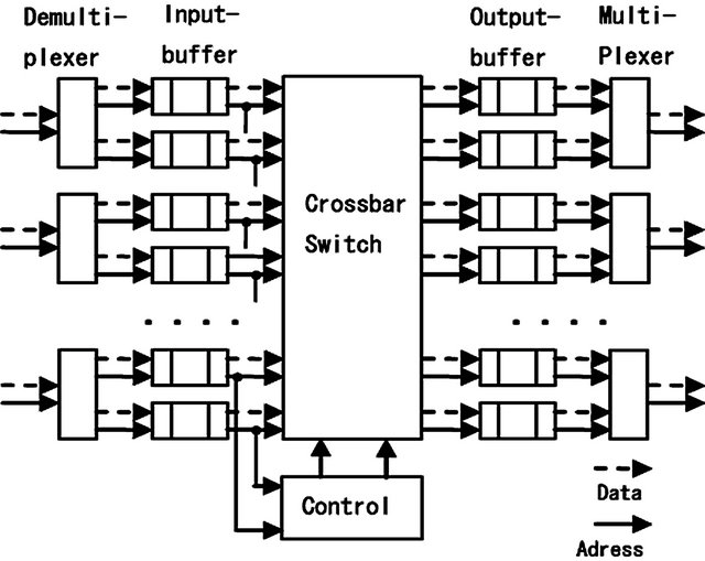
Figure 5. Router architecture.
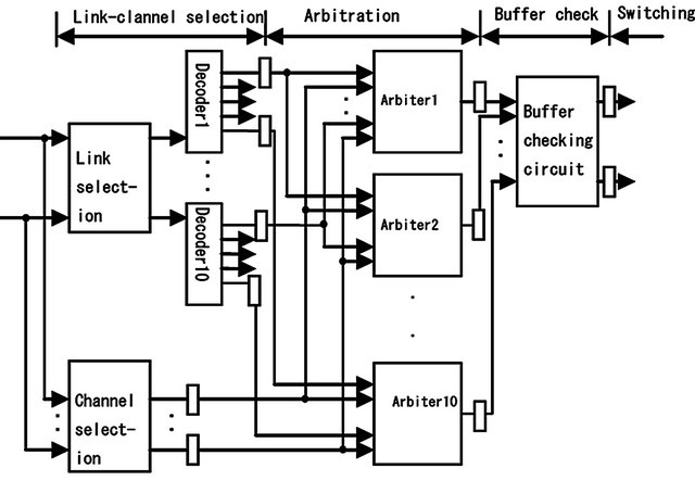
Figure 6. Router control block.
channel for a packet according to the header information. The delay can be estimated roughly by describing the selection function and discussing the complexity. The selection function assumes that the present PE and the channel number are constants and takes as its inputs the channel information (congested or uncongested) and header information (destination PE number etc.). The selection function is divided into channel selection function and link selection function. Channel selection function selects the channel and link selection function selects the link.
The selection function of deterministic routing in PEs at the corners of BMs is shown in Figure 7. The parts of this selection function that are different from Figure 7 for the CS and LS algorithms are shown in Figures 8 and 9, respectively. The part where the change is made are shown by the broken-line square. As shown in Figure 7, the selection function consists of link selection function selectlink and channel selection function selectchannel.
The link selection function is divided into selectlink, which determines whether the link to be selected will be an intra-BM or inter-BM link, and select_intra_link & route_higher_level_link, which select links from among the intra-BM and inter-BM links, respectively. Such a selection is done in every clock cycle. In the CS algorithm, only the channel selection function is changed, while in the LS algorithm, only route_higher_level_link function is changed. The changes add some IF statements. It is seen that only one IF statement is added in the LS algorithm. The delay is increased by the time for that IF statement. In the CS algorithm, three IF statements are added. However, they can be implemented in parallel using hardware, the delay is still only one IF statement time.
The implementation of the DDR algorithm is more complex. In the DDR algorithm, the output channel candidates are decided by the channel selection function, which depends on the output of the link selection function. It means that the channel candidates are decided after the link candidates have been decided by the link selection function. However, it is possible to process the channel selection and link selection functions in parallel and reduce the processing time. It also include the part of the link selection function in the channel selection unit. The increase of delay for the selection function is considerable in a complex algorithm. Because of the long delay of the DDR link selection function, we have implemented the output link decision circuits in parallel. Henceforth, this method is called parallel implementation; it increases the hardware cost but reduce the delay of the selection function.
Evaluation results are presented in the next section. For the implementation and evaluation, we used Xilinx Project Navigator and VirtexU (speed grade = 5) is used.
5.2. Hardware Cost Evaluation
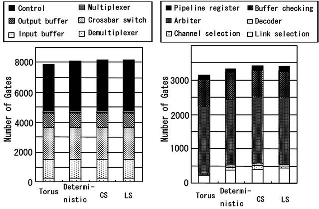
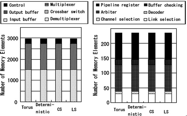
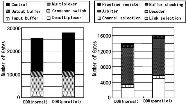
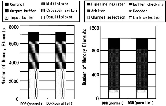
The hardware costs for the router of a TESH network are shown in Figures 10 and 11. The logic gate in this figure is a 4-input logic gate with arbitrary output. In these figures, the numbers of logic gates in the CS and LS algorithms are 1.1% and 0.7% higher than that of deterministic, dimension-order routing. The numbers of memory elements in the CS and LS algorithm are the same as in dimension-order routing. The hardware costs for the DDR algorithm are shown in Figures 12 and 13. The numbers of logic gates in the conventional and parallel implementations are 12.0% and 21.9% higher than that of dimension-order routing, and the numbers of memory elements are 13.9% higher than that of dimension-order routing. From these results, it is shown that the hardware cost of the CS and LS algorithms are almost equal to that of the dimension-order routing. There is a trivial difference in hardware cost among the routing algorithms. And the hardware cost of the DDR algorithm is slightly higher than that of dimension-order routing algorithm.
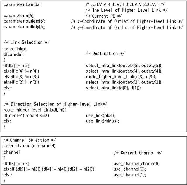
Figure 7. Selection function of dimension order routing.
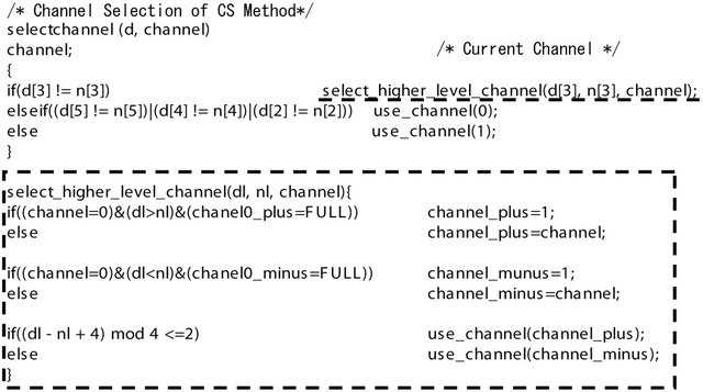
Figure 8. Selection function of CS routing.
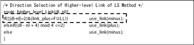
Figure 9. Selection function of LS routing.
 (a) (b)
Figure 10. Comparison of the number of logic gates in different router block of dimension-order, CS, and LS algorithms. (a) The whole circuit; (b) Control unit.
 (a) (b)
Figure 11. Comparison of the number of memory elements in different router block of dimension-order, CS, and LS algorithms. (a) The whole circuit; (b) Control unit.
 (a) (b)
Figure 12. Comparison of the number of logic gates in different router block of conventional and parallel DDR algorithms. (a) The whole circuit; (b) Control unit.
 (a) (b)
Figure 13. Comparison of the number of memory elements in different router block of conventional and parallel DDR algorithms. (a) The whole circuit; (b) Control unit.
6. Evaluation of Network Performance
6.1. Software Simulation
6.1.1. Simulation Environment
We have developed a wormhole routing simulator to evaluate dynamic communication performance of the TESH(2,3,0) network with 4096 PE. Dynamic communication performances are simulated for dimension-order routing algorithm, CS algorithm, LS algorithm, DDR algorithm, and combinations of them. Extensive simulations have been carried out for uniform and hotspot traffic patterns. The dynamic communication performance of an interconnection network is characterized by message latency and network throughput. Message latency refers to the time elapsed from the instant when the first flit is injected into the network from the source to the instant when the last flit of the message is received at the destination. Average transfer time is the average value of the latency for all packets. Network throughput refers to the maximum amount of information delivered per unit of time through the network. It is the average value of the number of flits which a PE receives in each clock cycle. In the evaluation of dynamic communication performance, flocks of messages are sent in the network to compete for the output channels. Packets are transmitted by the request-probability r during T clock cycles and the number of flits which reached at destination PE and its transfer time are recorded. Then the average transfer time and throughput are calculated and plotted as average transfer time in the horizontal axis and throughput in the vertical axis. The process of performance evaluation is carried out with changing the request-probability r.
The packet size is 16 flit and flits are transmitted for 20,000 cycles, i.e., T = 20,000. In each clock cycle, one flit is transferred from the input buffer to the output buffer, or from output to input if the corresponding buffer in the next node is empty. Therefore, transferring data between two nodes takes 2 clock cycles. Four virtual channels per physical channel are simulated, and they are arbitrated by a round-robin algorithm. The buffer length of each channel is 2 flits. In the DDR algorithm, the number of deterministic channel and adaptive channel are two respectively. In other algorithms, a pair of channels is used for deadlock avoidance, and two pairs are used to select channels. The transfer method of the packet is wormhole routing [16].
6.1.2. Uniform Traffic Pattern
In a uniform traffic, destinations are chosen randomly with equal probability among the nodes in the network. Figures 14 and 15 shows the average transfer time as a function of network throughput. The horizontal axis indicates network throughput and the vertical axis indicates transfer time. Also, the number inside the figure is the request-probability r. Each curve stands for a particular routing algorithm of the  network.
From Figure 14, it is seen that the maximum throughput of CS, LS, and combination of CS and LS (CS + LS) algorithms are higher than when the dimension-order routing algorithm is used. Also the maximum throughput of the CS + LS algorithm is higher than when the LS and CS algorithms are individually used. The average transfer time at zero load, called zero-load latency, of all the algorithms shown in Figure 14 are almost equal; because all the algorithms applied on  network. A packet never contends for network resources with other packets in zero load. As shown in Figure 15, it is seen that the maximum throughput of the algorithm with DDR is far higher than that of the algorithm without DDR. Another interesting point is that zero-load latency of the DDR algorithm is lower than zero-load latency of
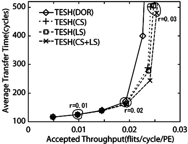
Figure 14. Comparison of dynamic communication performance of the TESH(2,3,0) network between dimensionorder, CS, LS, and CS + LS algorithms with uniform traffic pattern: 4096 nodes, 4 VCs, and 16 flits.
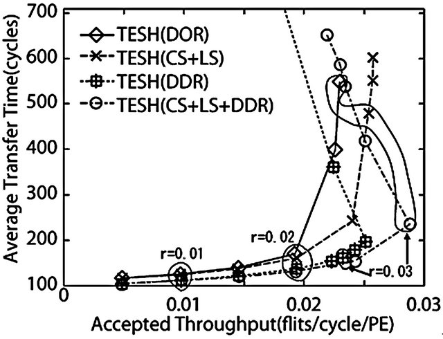
Figure 15. Comparison of dynamic communication performance of the TESH(2,3,0) network between dimensionorder, CS + LS, DDR, CS + LS + DDR algorithms with uniform traffic pattern: 4096 nodes, 4 VCs, and 16 flits.
the DDR algorithm is lower than that of other routing algorithms considered in this paper. The reason is that the transfer path of DDR is shorter than deterministic routing.
6.1.3. Hot-Spot Transfer
For generating hot spot traffic we used a model proposed by Pfister and Norton [19]. According to this model, each node first generates a random number. If that number is less than a predefined threshold, the message will be sent to the hot-spot PE. Otherwise, the message will be sent to other nodes, with a uniform distribution. In real application, it may happen that there are some packets (hot-spot packets) which remain in the network, and request rates are very high. Hot-spot packets go to the hot-spot . Here, the simulations were carried for the TESH network that Node
  are source PE and Node
  are hot-spot
 . The hot-spot flit generation probability are assumed to be
 , i.e., the hot-spot percentages are assumed to be 10%.
Figures 16 and 17 show the average transfer time as a function of network throughput for the hot-spot traffic patterns. The horizontal axis indicates network throughput, the vertical axis indicates average transfer time, and the number inside the figure is the requestprobability r. Each curve stands for a particular routing algorithm.
As depicted in Figure 16, the throughput of the dimension-order routing and CS algorithm are almost same. However, the throughput of LS algorithm is higher than that of dimension-order routing algorithm. As the packets can avoid congested links in LS algorithm, LS algorithm has an advantage in communication patterns which can create the congestion such as hot-spot traffic pattern. As depicted in Figure 17, the DDR algorithm has a low average transfer time in comparison with the other algorithms at zero-load like uniform traffic pattern. Also the maximum throughput of the DDR algorithm under hot-spot traffic pattern is higher than that of other algorithms. Because the choice of the inter-BM link is more than that of CS and LS algorithms. In this experiment, higher-level links of the neighborhood of destination PE are congested because hotspot packets use higher-level links intensively. Global adaptive routing algorithm such as DDR algorithm has an advantage in hot-spot traffic pattern because a lot of inter-BM links can be selected as compared with local adaptive routing. Therefore, with the hot-spot traffic pattern, the DDR algorithm yields better dynamic communication performance than that of dimension-order, LS, and CS algorithms.
6.2. Evaluation with Hardware Implementation
The delay time of each unit using two virtual channels is shown in Table 1 and using four virtual channels are shown in Table 2. As mentioned above, the delay time is divided into four pipelining stages, and the delays of stages  are as follows.
stage-1: 
stage-2: 
stage-3: 
stage-4: 
Here,  are the time delay of the link selection circuit, channel selection circuit, decoder,
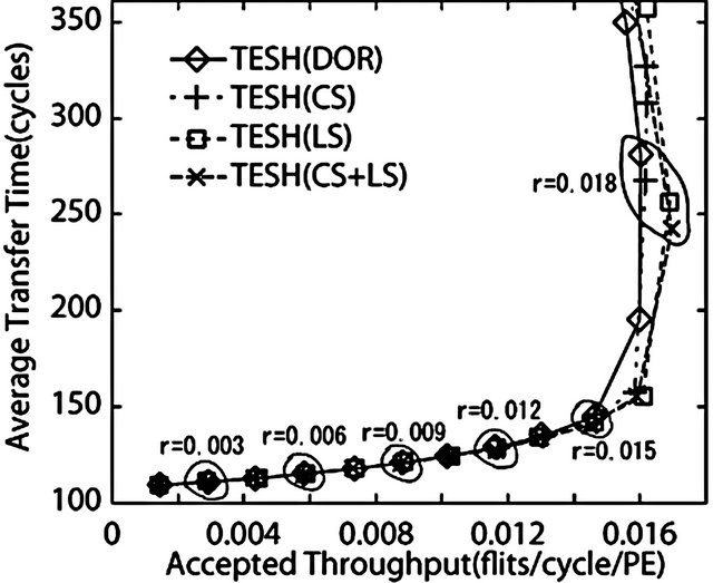
Figure 16. Comparison of dynamic communication performance of the TESH(2,3,0) network between dimensionorder, CS, LS, and CS + LS algorithms with hot-spot traffic pattern: 4096 nodes, 4 VCs, and 16 flits.
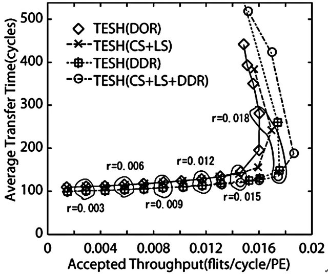
Figure 17. Comparison of dynamic communication performance of the TESH(2,3,0) network between dimensionorder, CS + LS, DDR, CS + LS + DDR algorithms with hotspot traffic pattern: 4096 nodes, 4 VCs, and 16 flits.
Table 1. Delay of control unit with 2 channels (ns).
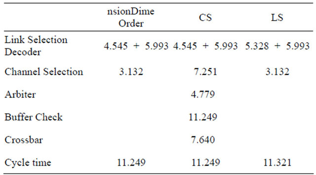
arbiter, buffer checking circuit, and crossbar switch, respectively. The maximum latency from stage-1 to stage-4 is the minimum clock time of the router. Since the link selection and channel selection circuits run at the
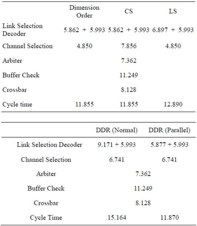
Table 2. Delay of control unit with 4 channels (ns).
same time in stage-1 of the control circuit, the delay of stage-1 is the larger value of  or
or .
.
TESH is a hierarchical network with complicated structure and the routing of message in this network is also complicated. The number of links and the number of virtual channels are 4 and 2, respectively in the CS and LS algorithms. Thus, the time delay for the CS and LS algorithms are the same to that of dimension-order routing after optimizing with a logic synthesis tool. With the normal implementation of the DDR algorithm, the minimum clock time is increased due to the large circuit delay of link selection. On the other hand in parallel implementation of the DDR algorithm, the influence on minimum clock time is small because the link selection circuit delay is decreased. This minimum clock cycle time is considered as single cycle time and is used for the dynamic communication performance evaluation.
Instead of simulation clock cycle the dynamic communication performance is evaluated in clock cycle time, i.e., in nano-second (ns). The minimum clock time is used for the evaluation of each routing algorithms. One cycle time is the minimum clock time of each algorithm. The average transfer time as a function of network throughput is portrayed in Figures 18 and 19 using uniform traffic pattern for two and four channels, respectively. The horizontal axis indicate network throughput, i.e., the average number of flits delivered through the network per unit time. The throughput is the number of delivered flits per PE in 1 ns, i.e., Flits/PE·ns.
As shown in Figure 18, the maximum throughput of the CS and LS algorithms on a TESH network is noticeably higher than that of the dimension-order routing. In the CS algorithm, there is no influence of channel selection circuit delay. In the LS algorithm, the delay is slightly high. However, the difference is trivial. As shown in Figure 19, the maximum throughput using normal implementation of DDR algorithm is lower than that of other algorithms. Due to complicated routing principle of DDR algorithm, its link selection circuit delay is large, which in turns make the clock cycle time of DDR algorithm long. On the other hand, the maximum throughput of parallel-implemented DDR algorithm is higher than that of other algorithms.
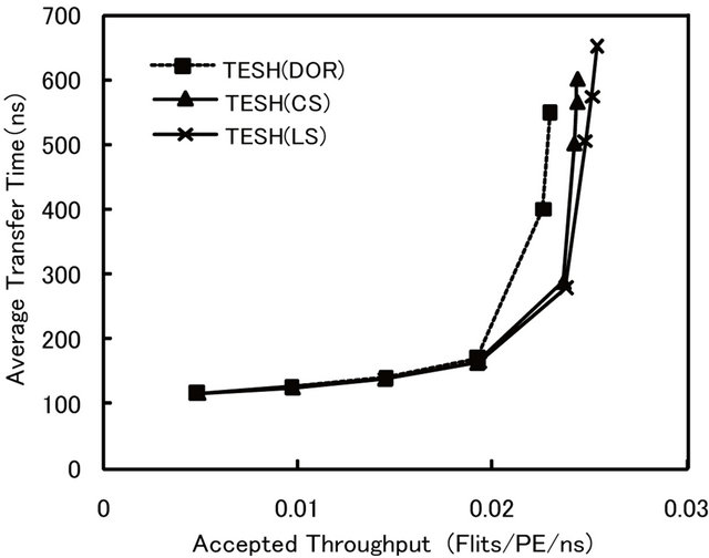
Figure 18. Comparison of dynamic communication performance of the TESH(2,3,0) network using hardware implemented router between dimension-order, CS, and LS algorithms with uniform traffic pattern: 4096 nodes, 2 VCs, and 16 flits.
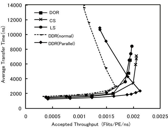
Figure 19. Comparison of dynamic communication performance of the TESH(2,3,0) network using hardware implemented router between dimension-order, CS, LS, and DDR algorithms with uniform traffic pattern: 4096 nodes, 4 VCs, and 16 flits.
7. Conclusions
We have proposed three adaptive routing algorithms, CS, LS, DDR along with dimension-order routing with their hardware implementation for the TESH network. The proposed algorithms are simple and efficient for using the virtual channels, physical links, and direction of network to improve dynamic communication performance. In this paper, we have evaluated the delay and hardware cost of the proposed routing algorithm using VHDL. The logic gates of the CS and LS algorithms are almost equal and the memory elements of the CS and LS algorithms are exactly equal to that of dimension-order routing. The logic gates and memory elements of the DDR algorithm are slightly higher than that of dimension-order routing.
Using the routing algorithms described in this paper and with uniform and hot-spot traffic patterns, we have evaluated the dynamic communication performance of a TESH network. The average transfer time at zero-load of the TESH network using the DDR algorithm is noticeably lower than when the dimension-order routing is used. On the other hand, maximum throughput using the CS, LS, and DDR algorithms is higher than when the dimension-order routing is used. A comparison of dynamic communication performance reveals that the DDR algorithm outperforms all other algorithms; a TESH network using the DDR algorithm yields low latency and high throughput, which are indispensable for the high performance of massively parallel computing system. Using the clock time selected by minimum cycle time through hardware implementation of each routing algorithms, we have also evaluated the communication performance. It is shown that the dynamic communication performance of a TESH network using CS, LS, DDR algorithms are higher than that of dimension order routing. Among them DDR algorithm yields the highest communication performance.
REFERENCES
- W. J. Dally, “Performance Analysis of k-Ary n-Cube Interconnection Networks,” IEEE Transactions on Computers, Vol. 39, No. 6, 1990, pp. 775-785. doi:10.1109/12.53599
- V. K. Jain, T. Ghirmai and S. Horiguchi, “TESH: A New Hierarchical Interconnection Network for Massively Parallel Computing,” IEICE Transactions on Information and Systems, Vol. E80-D, No. 9, 1997, pp. 837-846.
- V. K. Jain, T. Ghirmai and S. Horiguchi, “Reconfiguration and Yield for TESH: A New Hierarchical Interconnection Network for 3-D Integration,” IEEE Proceedings of International Conference Wafer Scale Integration, Austin, 9-11 October 1996, pp. 288-297.
- V. K. Jain and S. Horiguchi, “VLSI Considerations for TESH: A New Hierarchical Interconnection Network for 3-D Integration,” IEEE Transactions on VLSI Systems, Vol. 6, No. 3, 1998, pp. 346-353. doi:10.1109/92.711306
- S. Bhansali, et al., “3D Heterogeneous Sensor System on a Chip for Defense and Security Applications,” Proceedings of the SPIE Defense and Security Symposium (DSS), Vol. 5417, 2004, pp. 413-424.
- G. H. Chapman, V. K. Jain and S. Bhansali, “Defect Avoidance in 3-D Heterogeneous Sensor,” Proceedings of the 1992 IEEE International Symposium on Defect and Fault Tolerance in VLSI Systems (DFT’04), Cannes, 10-13 October 2005, pp. 67-75.
- Y. Miura and S. Horiguchi, “A Deadlock-Free Routing for Hierarchical Interconnection Network: TESH,” Proceedings of the 4th International Conference on High Performance Computing in Asia-Pacific Region, Beijing, 14-17 May 2000, pp. 128-133. doi:10.1109/HPC.2000.846532
- W. J. Dally, “Virtual-Channel Flow Control,” IEEE Transactions on Parallel and Distributed Systems, Vol. 3, No. 2, 1992, pp. 194-205. doi:10.1109/71.127260
- C. S. Yang and Y. M. Tsai, “Adaptive Routing in k-Ary n-Cube Multicomputers,” Proceedings of ICPADS’96, Tokyo, 3-6 June 1996, pp. 404-411.
- W. J. Dally and C. L. Seitz, “Deadlock-Free Message Routing in Multiprocessor inter-connection Networks,” IEEE Transactions on Computers, Vol. C-36, No. 5, 1987, pp. 547-553. doi:10.1109/TC.1987.1676939
- W. J. Dally and H. Aoki, “Deadlock-Free Adaptive Routing in Multicomputer Networks Using Virtual Channels,” IEEE Transactions on Parallel and Distributed Systems, Vol. 4, No. 4, 1993, pp. 466-475. doi:10.1109/71.219761
- C. J. Glass and L. M. Ni, “Maximally Fully Adaptive Routing in 2D Meshes,” Proceedings of the 1992 International Conference on Parallel Processing, An Arbor, 17-21 August 1992, pp. 101-104.
- J. Duato, “A New Theory of Deadlock-Free Adaptive Routing in Wormhole Networks,” IEEE Transactions on Parallel and Distributed Systems, Vol. 4, No. 12, 1993, pp. 1320-1331. doi:10.1109/71.250114
- Y. Miura and S. Horiguchi, “An Adaptive Routing for Hierarchical Interconnection Network TESH,” Proceedings of the 3rd International Conference on Parallel And Distributed Computing, Applications and Technologies, Kanazawa, 3-6 September 2002, pp. 335-342.
- Y. Miura, M. Kaneko and S. Horiguchi, “Examination of Hardware Implementation on Adaptive Routing for Hierarchical Interconnection Network TESH,” Proceedings of International Workshop on High Performance and Highly Survivable Routers and Networks (HPSRN 2008), Sendai, 13-14 March 2008, pp. 17-30.
- L. M. Ni and P. K. McKinley, “A Survey of Wormhole Routing Techniques in Direct Networks,” Proceedings of the IEEE, Vol. 81, No. 2, pp. 62-76, 1993.
- A. Kumary, P. Kunduz, A. P. Singhx, L.-S. Pehy and N. K. Jhay, “A 4.6T bits/s 3.6 GHz Single-Cycle NoC Router with a Novel Switch Allocator in 65 nm CMOS,” 25th International Conference on Computer Design (ICCD 2007), Lake Tahoe, 7-10 October 2007, pp. 63-70. doi:10.1109/ICCD.2007.4601881
- M. Koibuchi, K. Anjo, Y. Yamada, A. Jouraku and H. Amano, “A Simple Data Transfer Technique Using Local Address for Networks-on-Chips,” IEEE Transactions on Parallel and Distributed Systems, Vol. 17, No. 12, 2006, pp. 1425-1437. doi:10.1109/TPDS.2006.166
- G. F. Pfister and V. A. Norton, “Hot Spot Contention and Combining in Multistage Interconnection Networks,” IEEE Transactions on Computers, Vol. 34, No. 10, 1985, pp. 943-948. doi:10.1109/TC.1985.6312198