World Journal of Mechanics
Vol.4 No.1(2014), Article ID:42386,6 pages DOI:10.4236/wjm.2014.41004
The Calculation of Stress-Strain State of Anisotropic Composite Finite-Element Area with Different Boundary Conditions on the Surface
Druzbi Narodov Prospectus 27/44, Kyiv, Ukraine
Email: bergulyov@yandex.ru
Received October 17, 2013; revised November 23, 2013; accepted December 18, 2013
ABSTRACT
The numerical analytic research approach of stress-strain state of anisotropic composite finite element area with different boundary conditions on the surface, is represented below. The problem is solved by using a spatial model of the elasticity theory. Differential equation system in partial derivatives reduces to one-dimensional problem using spline collocation method in two coordinate directions. Boundary problem for the system of ordinary higher-order differential equation is solved by using the stable numerical technique of discrete orthogonalization.
Keywords:Composite Finite-Element Areas; Boundary Conditions; Elasticity Theory; Spline Approximation; Collocation Methods
1. Introduction
Composite finite-element areas have widespread application in many fields of modern technology, such as shipbuilding, space industry, construction building etc. An important issue in terms of providing obdurability when exploiting relevant construction elements, is the matter of obtaining information about their stress-strain state. The pursuance of the research on the basis of the elasticity theory spatial model of the finite element composite areas of arbitrary shape, is connected with calculation problems. That’s why one can find limited number of scientific works on the subject.
Here we suggest an effective numerical analytic research approach of stress-strain state of the layered anisotropic finite-element areas on the basis of the elasticity theory. The approach is based upon using the spline approximation and collocation methods, which helps us to reduce our space boundary problem for differential equation in partial derivatives systems to the corresponding problem for ordinary differential equations. The latter is solved by using the stable numerical technique of discrete orthogonalization.
2. Basic Equations
Let K denote the anisotropic plate composed of conjoined cubic plates (Figure 1).
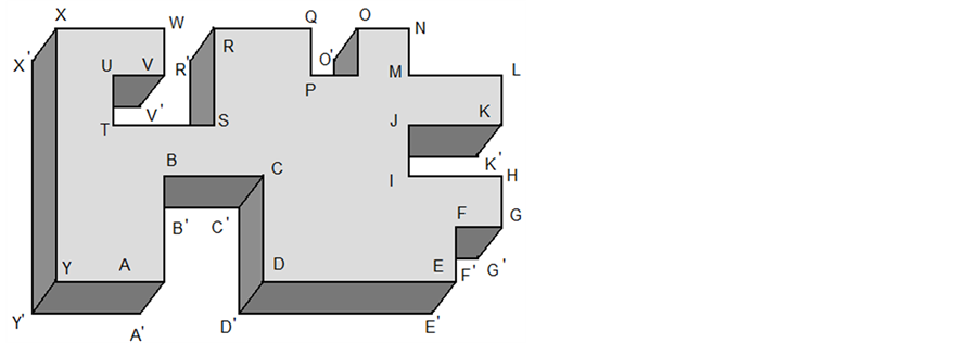
Figure 1. Anisotropic plate composed of conjoined cubic plates.
Let us consider the stress-strain state problem of such fixed thickness plate in a rectangular coordinate system (X, Y, Z). According to the linear elastic theory, original equations will appear as follows:
Equilibrium equations:
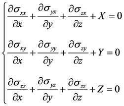 (1)
(1)
Where
![]() follows the pairing tangent stress law:
follows the pairing tangent stress law:
![]()
Cauchy equations:
 (2)
(2)
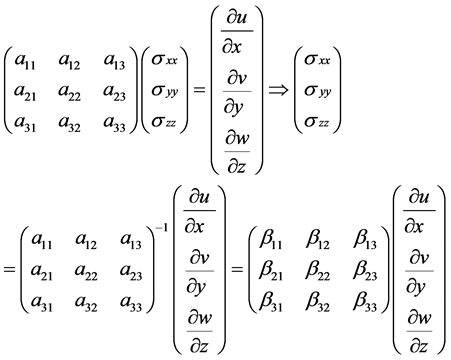
Physical equations expressing Hooke’s law for anisotropic material:
 (3)
(3)
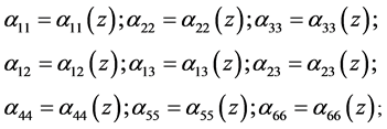
As we see, twenty one independent components occur in formula (3). Generally in practice, the objects under consideration have only one plane of elastic symmetry tangent to the coordinate surface z = const. In this situation, the number of explanatory variables is equal to thirteen, and Hooke’s law for such objects changes to:
 (4)
(4)
Coefficients
![]() of this system are determined from:
of this system are determined from:
 (5)
(5)

In these evaluations:
 ,
,
![]() ,
, —elasticity modulus in x, y, z-directions respectively;
![]() —shear modulus for the planes parallel to coordinate planes x = const, y = const, z = const respectively;
—shear modulus for the planes parallel to coordinate planes x = const, y = const, z = const respectively;
![]() ,
,
![]() ,
,
![]() ,
,
![]() ,
,
![]() ,
,![]() —Poisson’s ratios characterizing lateral contraction when stretched along the coordinate axes;
—Poisson’s ratios characterizing lateral contraction when stretched along the coordinate axes;![]() ,
,![]() —ratios characterizing shears in the planes parallel to the coordinate planes, resulting from shearing stresses that the planes tangent to other coordinate planes experience.
—ratios characterizing shears in the planes parallel to the coordinate planes, resulting from shearing stresses that the planes tangent to other coordinate planes experience.![]() ,
,![]() —coefficients of mutual influence characterizing shears in coordinate planes, due to normal stresses;
—coefficients of mutual influence characterizing shears in coordinate planes, due to normal stresses;
![]() ,
,
![]() ,
,![]() —coefficients of mutual influence characterizing expansions in length due to shear stress.
—coefficients of mutual influence characterizing expansions in length due to shear stress.
Further, by applying elementary transformations we obtain resolving system of three second-order partial differential equations describing the stress-strain state of the plate from the systems (1), (2), (4):

 (6)
(6)

Coefficients
 in system (6), are determined by the mechanical characteristics of the material, taking into account ratios (5).
In practice, the formulas for the anisotropic object with a single plane elastic symmetry, are developed from the formulas for the orthotropic object by rotating the coordinate system by an angle
 about axis OZ.
In this connection, the coefficients of the elastic compliance matrixes![]() и
и![]() are in both cases interrelated by the following formulas:
are in both cases interrelated by the following formulas:
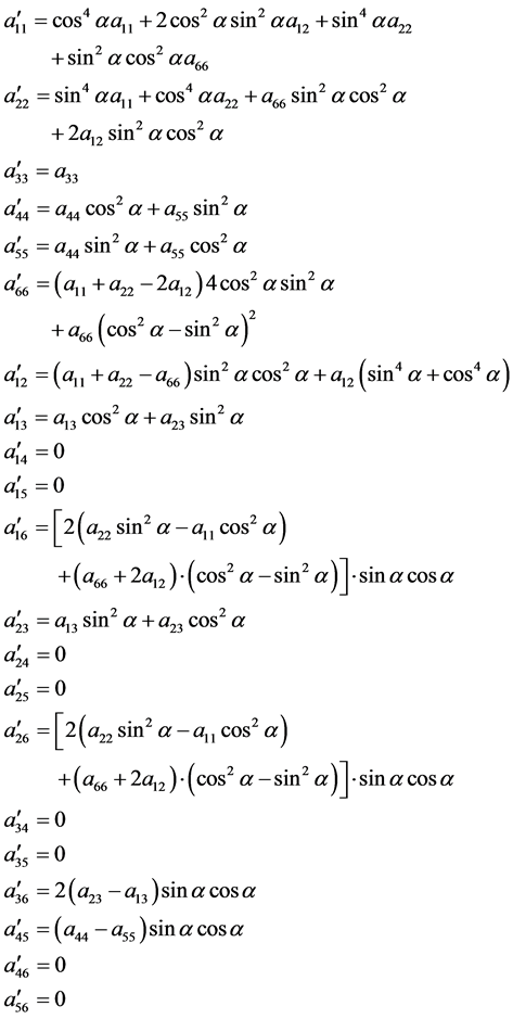 (7)
(7)
By this means, knowing coefficients
![]() for an orthotropic object and the angle of rotation we can formulate a well-posed problem for the anisotropic object with a single plane of elastic symmetry.
for an orthotropic object and the angle of rotation we can formulate a well-posed problem for the anisotropic object with a single plane of elastic symmetry.
The solution of (6) will be sought in the form of (8)
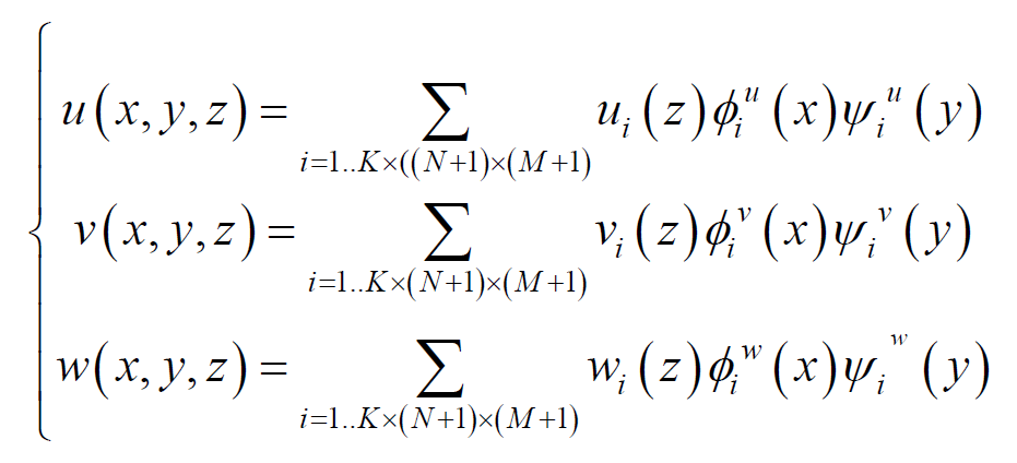 (8)
(8)
Here: N, M—the dimension of the collocation grid for each cubical plate. K—the number of cubic subplates of the plate [1].
3. Statement of the Boundary Conditions
Let’s consider cubic component of the plate [1] (Figure 2). Given normal and sheer stresses
 on faces z = 0, z = 1, that will determine distribution of stresses, strains and shifts within a thick-walled plate.
One can express from the set of Equations (2), (4) that:

In matrix shape, the system is of the form:
 (9)
(9)
i.e.:

Shear stresses may be defined as follows:

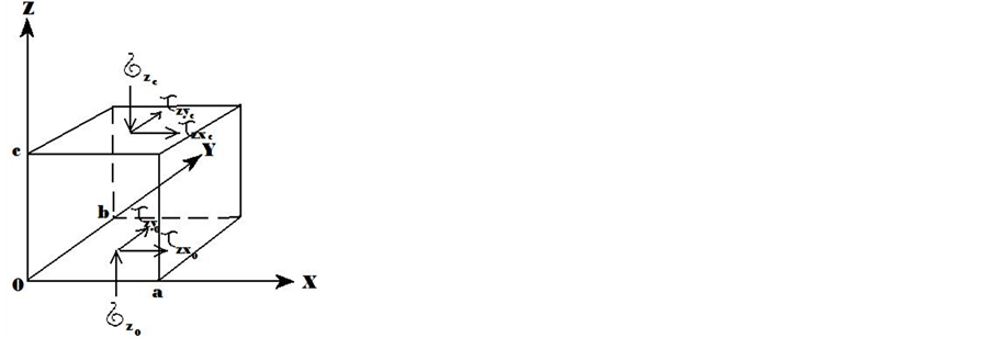
Figure 2. Boundary conditions.
Thus, boundary conditions on the faces z = 0, z = c are described by the system:
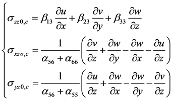 (10)
(10)
Approximation of solutions of the system (10), is performed with the help of functions (8).
Boundary conditions of three types, can be set on the lateral faces: conditions, corresponding to rigidly fixed contour, conditions, corresponding to simply supported contour, conditions for free contour. Approximations of these boundary conditions is achieved by fitting B3 spline coefficients, which determine
 functions.
 functions, will be sought in the form of:
 (11)
(11)
 (12)
(12)
Let’s consider the cubic component of the plate as an example [2] (Figure 2) and boundary conditions on x = 0 face in case of rigidly fixed and simply supported contours.
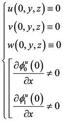
3.1. Rigidly Fixed Contour
This case corresponds to the conditions:
 (13)
(13)
Let’s define
![]() from the formula (9)
from the formula (9)

As , it follows that:
 . Then, for fulfillment
 condition, it’s necessary and sufficient for
 condition to be met. (14)
It follows that:

The latter equation follows from
 . Therefore, it is sufficient for at least one of the
 values not to be equal to zero simultaneously, to satisfy the condition (14).
I.e., the conditions (13), can be replaced by the conditions:
 (15)
(15)
For the conditions (15) fulfillment is sufficient to satisfy the system:
 (16)
(16)
For this, we choose the coefficients:
 (17)
(17)
Taking into consideration that:
 (18)
(18)
We obtain:

As we can see, selected in the form of (17), the coefficients satisfy the system (16), which automatically causes the conditions (13) fulfillment. Thus, for rigidly fixed contours x = 0,
 functions take on form:
 (19)
(19)
 (20)
(20)
3.2. Simply Supported Contour
This case satisfies the conditions:
 (21)
(21)
From the preceding considerations it is seen, that
 conditions can be replaced by

condition. For this case, we set the coefficients:
 (22)
(22)
 (23)
(23)
For specified coefficients according to (22), (23), we have:


As one can see, the coefficients can to satisfy the boundary conditions (21) if selected in the form of (22), (23). Therefore, for the simply supported x = 0 contour,
 functions take on the form:
 (24)
(24)
 (25)
(25)
And
 functions:
 (26)
(26)
 (27)
(27)
The boundary conditions for the free contour are defined similarly.
3.3. The Case of Non-Homogenous Orthotropic Material
In the case of non-homogenous Z-coordinate orthotropic material, stiffness properties characterizing stress-strain state of such plate, will take the form:
 -elasticity modulus in x, y, z-directions respectively;
 -elasticity modulus for the planes, parallel to
 planes respectively.
In this case, the coefficients of the elastic compliance matrix assume the form:
 (28)
(28)
After that, we have the system of three partial differential equations of the second order, which describes the stress-strain state of thick-walled rectangular orthotropic non-homogenous in Z-coordinate plate:
 (29)
(29)
 coefficients are defined by the coefficients of the elastic compliance matrix, described by the formulas (28).
If the material is non-homogenous in three spatial coordinates, the coefficients of the system (29) are the coefficients of all three spatial coordinates:

4. Statement of the Problem
Let us consider a simple-connected body of arbitrary shape with an arbitrary mounting on the subsurfaces. Let T denote it. We will consider it in the Cartesian XYZ reference system. The problem is to find the stress-strain state of the current object, consisting of an arbitrary material composition, with an arbitrary mounting on the surface, at an arbitrary load on it (steady or point load) and with arbitrarily given volumetric forces (weight, thermal expansion etc.).
5. Solution Procedure
Let us arrange the considered object T in the Cartesian reference system in such a way to make XOY, XOZ, YOZ planes tangent to the object, and each point of the object
 satisfy the condition
![]() (Figure 3). Consider the case of a composite layered object. We divide the object into horizontal layers, with the lower and upper bounds that are parallel to XOY plane. Each of these layers is approximated by cubic subplates (Figure 1). Stress-strain state of K-area, thus obtained, will be described by the formulas (6), (10), (13), (21). The boundary conditions at the joining point will be predetermined by the formulas:
(Figure 3). Consider the case of a composite layered object. We divide the object into horizontal layers, with the lower and upper bounds that are parallel to XOY plane. Each of these layers is approximated by cubic subplates (Figure 1). Stress-strain state of K-area, thus obtained, will be described by the formulas (6), (10), (13), (21). The boundary conditions at the joining point will be predetermined by the formulas:
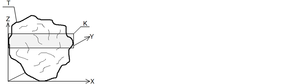
Figure 3. Simple-connected body of arbitrary shape with an arbitrary mounting on the subsurfaces.
 (30)
(30)
After the approximation of the required displacement functions in the form of (8), we obtain the system of ordinary differential equations of the following order:
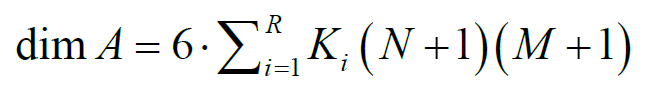 (31)
(31)
Here: R—the number of layers of the simple-connected T-object, —the number of cubic subplates in the layer,
 —the number of the spline collocation points per direction. The problem can be solved by using the stable numerical technique of discrete orthogonalization [1, 2].
6. Conclusion
This paper presents the numerical-analytic approach to solving the stress-strain state problems of an arbitrary finite element simple-connected composite object with different surface mounting types. The problem is solved by using the elasticity theory spatial model. Differential equation system in partial derivatives reduces to onedimensional problem using spline collocation method in two coordinate directions. End problem of ordinary higher-order differential equation system is solved by using the stable numerical technique of discrete orthogonalization [1, 2].
REFERENCES
- A. Y. Grigorenko, A. S Bergulyov and S. N. Yaremchenko, “The Solution of the Spatial Boundary Value Problems about Rectangular Plates Bending,” Proceedings of the National Academy of Sciences of Ukraine No. 10, 2010, pp. 44-51.
- A. Y. Grigorenko, A. S Bergulyov and S. N. Yaremchenko, “Third-Dimensional Boundary Value Problem Solution for the Bend of Rectangular Disks,” Reports of the National academy of sciences of Ukraine, No. 10, pp. 44-51.