World Journal of Mechanics
Vol. 3 No. 2 (2013) , Article ID: 30867 , 17 pages DOI:10.4236/wjm.2013.32010
Development of Analytical Model for Modular Tank Vehicle Carrying Liquid Cargo
1Department of Applied Sciences, University of Quebec at Chicoutimi, Saguenay, Canada
2Department of Mechanical Engineering, Laval University, Quebec, Canada
Email: *mbouazar@uqac.ca
Copyright © 2013 Messaoud Toumi et al. This is an open access article distributed under the Creative Commons Attribution License, which permits unrestricted use, distribution, and reproduction in any medium, provided the original work is properly cited.
Received February 27, 2013; revised April 8, 2013; accepted April 15, 2013
Keywords: Analytical Model; Tank Vehicle; Stability; Dynamic Behavior; Suspension
ABSTRACT
The study of dynamics of tank vehicles carrying liquid fuel cargo is complex. The forces and moments due to liquid sloshing create serious problems related to the instability of tank vehicles. In this paper, a complete analytical model of a modular tank vehicle has been developed. The model included all the vehicle systems and subsystems. Simulation results obtained using this model was compared with those obtained using the popular TruckSim software. The comparison proved the validity of the assumptions used in the analytical model and showed a good correlation under single or double lane change and turning manoeuvers.
1. Introduction
In general, numerical models are developed to understand the liquid sloshing phenomenon coupled with tank structure. They are able to determine the coupling behavior, only under specific conditions, such as periodic accelerations. The effects of suspension system, tire and road excitation on a moving vehicle have not been taken into consideration. Regarding the vehicle itself, different simple models for tractors and trailers have been described in literatures to study the dynamic behavior of heavy vehicles during various maneuvers. Ellis [1] developed a simple model for tractor-trailer type bicycle with four degrees of freedom where the load transfer was modeled using an additional degree of freedom (rolling motion). Hyun [2] adopted a model for vehicle with four degrees of freedom for the active control of roll-over of heavy vehicles. While various solid-liquid models have been developed to determine the dynamic behavior of vehicles carrying liquids, few models have been developed to reflect the effects of vehicle systems and subsystems, such as suspension and tire components. The models adopted for the vehicle systems are all based on simplified assumptions.
It is necessary to develop a comprehensive model because a vehicle is composed of various subsystems and the effects of those need to be considered. AutoSim package, one of most popular software for modeling of the behavior of a vehicle, was developed at the University of Michigan [3,4]. Three software applications were created based on the AutoSim package [5]. These software applications are CarSim, TruckSim and BikeSim for cars, heavy vehicles and motorcycles respectively. However, the TruckSim software does not include the effects of motion of a moving load [6-8]. They are easy to use for conventional vehicles only. However, they offer some models for unconventional designs and the models find applications in some specific research projects. Another drawback with these tools is that they work in a closed environment. Therefore the present work focussed on development of custom made models.
2. Vehicle Kinematic
To develop the model of the vehicle, there are several methods that could be exploited to derive the equations of motion such as Lagrange, Newton and virtual work methods. The popular alternative approach for dynamic modelling of vehicles is to use of simple models having a reasonable excution time. In this study, a new model was developed based on the simplified Ervin model [4]. This model was solved without any mathematical approximation and it took care of the complexity of liquid motion inside the tank. The solutions of the equations were obtained using the mathematical software Maple [9]. The equations were derived based on the principles of Newtonian mechanics and conservation of linear and angular momentums for a solid body.
2.1. Coordinate System
The large number of degrees of freedom for translation and rotational motion, required to represent an articulated vehicle, excludes the use of a single coordinate system. In fact, the equations of motion can be written more easily if several coordinate systems are employed. The purpose of this section is to identify the orientation of the various coordinate systems, and specify the variables required to connect the processing unit vectors in the various systems. The inertial coordinate system, the body coordinate system fixed to the sprung mass and the coordinate system fixed to the unsprung mass were used to describe the system. Newton’s laws are valid only for a finite acceleration in an inertial coordinate system . The orientations of coordinate axes were expressed in accordance with the Society of Automotive Engineers’ standard (SAE), where the positive x axis points anterior, the positive y axis is oriented to the right and the positive z axis points downward. In our model, each sprung mass was represented as a rigid body with six degrees of freedom namely, longitudinal, lateral, vertical, roll, pitch and yaw. For the unsprung mass, there were assigned two degrees of freedom namely, the roll and vertical motions relative to the point of attachment of the sprung mass. The equations were formulated such that there was no limit to the number of sprung and unsprung masses. All the equations were solved, without any mathematical simplification, using the symbolic computational software Maple [9].
Three coordinate systems were used to develop the equations of motion. The first one was attached to the inertial system , the second one was attached to each sprung mass
  and the third one was attached to each unsprung mass
 . Figure 1
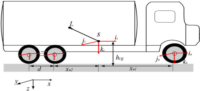
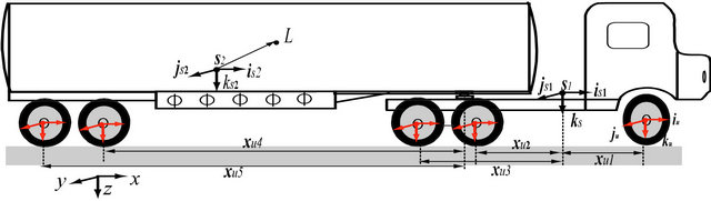
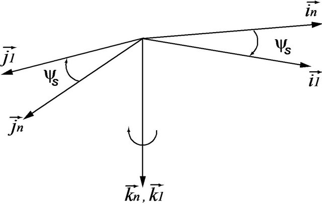
Figure 1. Fixed unit and articulated tank vehicles.
shows the coordinate systems for fixed unit and articulated vehicles.
2.1.1. Coordinate System Fixed to the Sprung Mass
The three rotational motions of the sprung mass were expressed by the three Euler angles: yaw  (around axis
 ), pitch
  (around axis
 ) and rolling motion
  (around axis
 ) as shown by Figure 2.
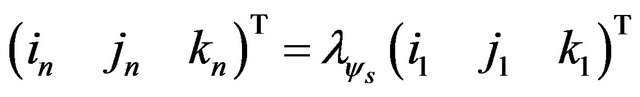
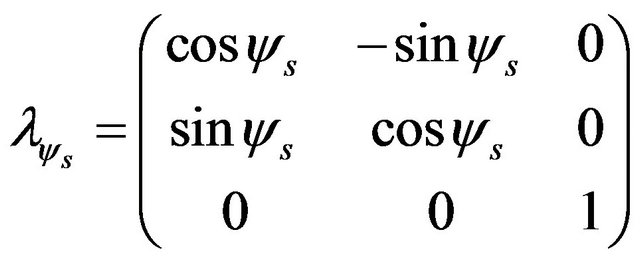
The transformation matrix between inertial system and the system fixed to the sprung mass was defined separately for the three successive rotations: yaw, pitch and roll.
Yaw :
:

 (1)
(1)
Pitch :
:
 (a)
(a)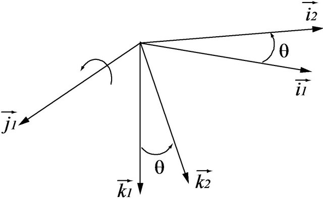 (b)
(b) (c)
(c)
Figure 2. (a) Yaw: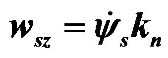 ; (b) Pitch:
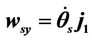 ; (c) Roll:
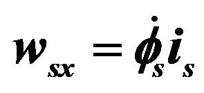 . Sprung mass orientation defined by euler angles.
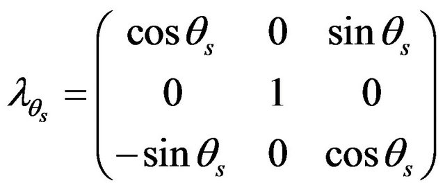 (2)
(2)
Roll :
:
 (3)
(3)
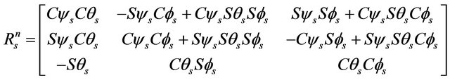
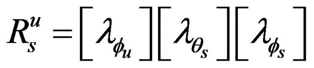
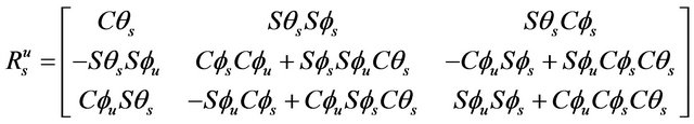
The transformation matrix, connecting the inertial system and the system fixed to the sprung mass, was obtained by combining the three matrices as follows:
 (4)
(4)
where: (please see Equation (5) below)
and:
 (6)
(6)
with index ( ,
, ).
).
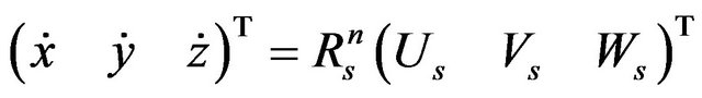
2.1.2. Linear and Angular Velocities of the Sprung Mass
The equations of motion of each sprung mass were developed and written for the system fixed to the sprung mass in terms of linear velocity  and angular velocity
  of the center of mass of the sprung mass. In order to calculate the velocity and Euler angles, expressions connecting the linear and angular velocities for both the systems were developed.
 (7)
(7)
 (8)
(8)
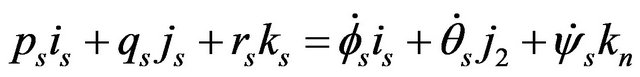
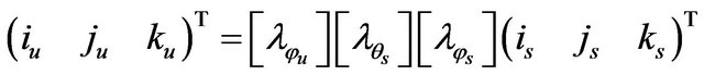
Introducing the transformation matrices between the two systems, the relationship between the angular velocities can be calculated by the following equations:
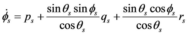
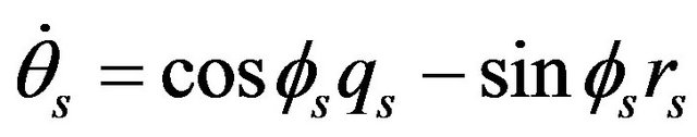 (9)
(9)
2.1.3. Coordinate System Fixed to the Unsprung Mass
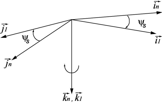
As mentioned earlier, two motions were assigned to each unsprung mass, namely, the roll motion and vertical motion relative to the sprung mass. It may be noted that the pitching motion of the unsprung mass, representing the axle of vehicle, is infinitely small and can be neglected [3]. The orientation of the sprung mass relative to the inertial coordinate system was defined by two rotational motions namely, yaw motion  and roll motion
  as illustrated in Figure 3.
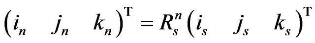
The transformation matrix between the system fixed to the unsprung mass and the inertial system can be expressed as:
Yaw :
:
 (10)
(10)
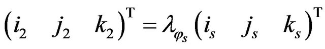
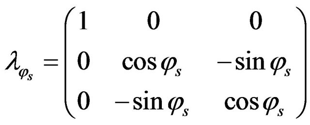
Roll :
:
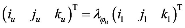
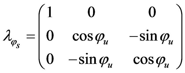 (11)
(11)
 (a)
(a)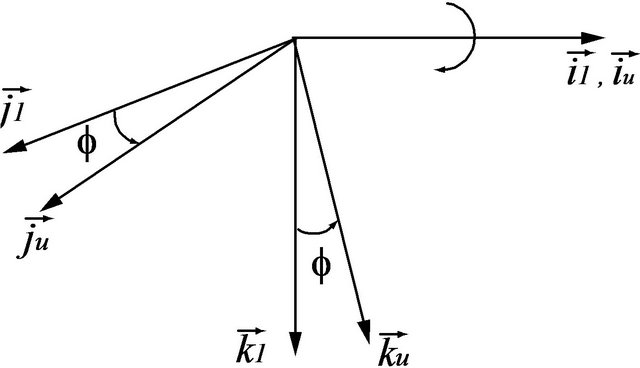 (b)
(b)
Figure 3. (a) Yaw; (b) Roll . Unsprung mass orientation defined by Euler angles.
 (5)
(5)
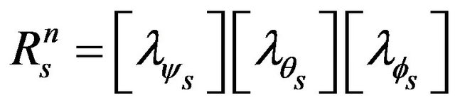
Therefore, the transformation matrix, that connects the system fixed to the unsprung mass and the inertial system, can be obtained by combining the above two transformations ((10) and (11)).
 (12)
(12)
The angular velocity of the unsprung mass can be defined by the following equation:
 (13)
(13)
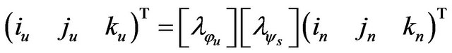
By introducing the transformation matrices between the inertial system and the system fixed to the unsprung mass, the angular velocity was expressed in terms of Euler angles as follows:
 (14)
(14)
On the other hand, the road excitation forces are in contact with the unsprung mass. These forces are transferred to the sprung mass through the suspension system. Therefore, the transformation matrix between the two systems fixed to the sprung and unsprung masses needs to be calculated.
 (15)
(15)
 (16)
(16)
where: (please see Equation (17) below).
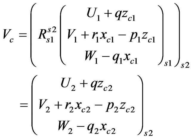
2.2. Sprung Mass Kinematics
For the derivation of equations of motion of the vehicle it is necessary to calculate the expression for the acceleration of an arbitrary point on the vehicle. Figure 4 shows  as the coordinate system fixed to the road (inertial) and
  as the system of the body coordinate with a
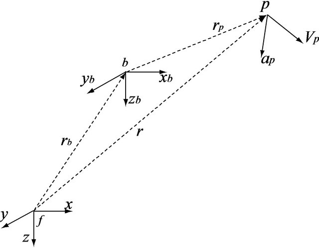
Figure 4. Coordinate systems.
translational velocity  and an angular velocity
 . For a given vector
 , the following expression [10] was obtained:
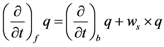 (18)
(18)
The indices f and b indicate that the derivative was calculated with respect to the inertial system and system of the body concerned respectively.
The velocity of point p in the vehicle, relative to inertial system, can be calculated by the following expression:
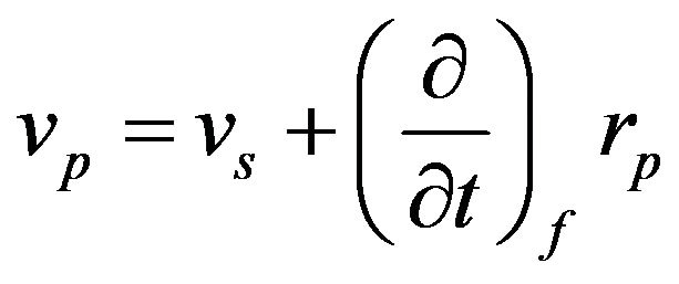 (19)
(19)
Therefore, substitution of Equation (18) in Equation (19) gives:
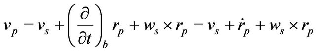 (20)
(20)
The acceleration of the point  can be calculated by differentiating Equation (20) with respect to time:
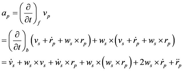 (21)
(21)
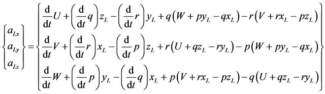
Since the center of mass of the sprung mass coincides with the origin of the coordinate system attached to the sprung mass, acceleration of the center of mass of the sprung mass was obtained by replacing  in Equation (21):
 .
.
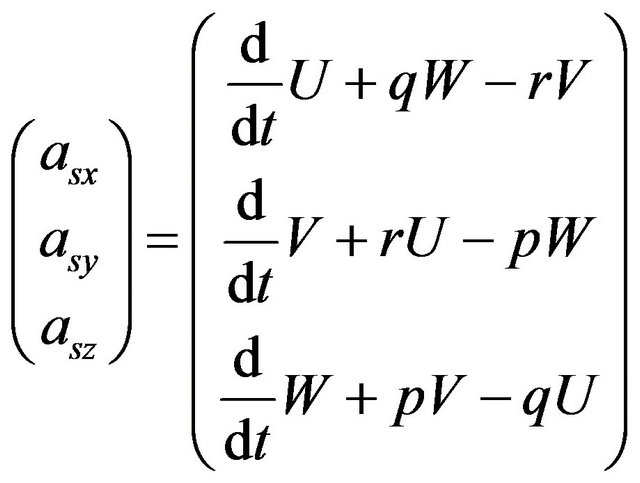 (22)
(22)
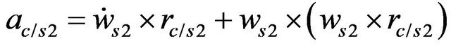
In this study, it was assumed that the load of the liquid, represented by the center of mass, can move as a material point and can be represented by a remote vector 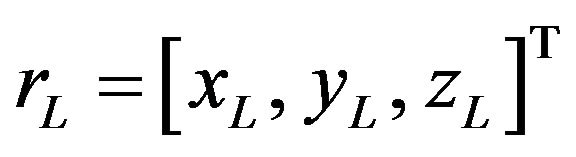 from the center of mass of the sprung mass with the same angular velocity
  as that of the sprung mass of the vehicle as shown in Figure 5.
 (17)
(17)
Hence, the acceleration of the center of mass of the liquid can be obtained by replacing the expression  in Equation (21). Moreover, in this study the interaction between the vehicle and the liquid was modeled as a multi-body system using small time step
 . As the coordinates of the vector
  were updated at each time step, the relative velocity and acceleration relative to the coordinate system fixed to the sprung mass were neglected.
 (23)
(23)
2.3. Unsprung Mass Kinematics
The position of the unsprung mass is located in relation to the point where the sprung mass is attached as shown in Figures 5 and 6.
 (24)
(24)
where:
 : represents the position of center of sprung mass from the inertial system.
 : represents the position of the roll center relative to the system fixed to the sprung mass.
 : represents the position of the roll center relative to the system attached to the unsprung mass. The velocity was calculated by differentiating Equation (24) with respect to time:
 (25)
(25)
The acceleration was calculated by differentiating Equation (25) with respect to time:
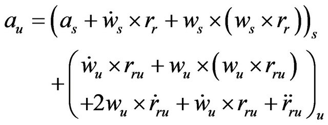 (26)
(26)
where suffixes  and
and  indicate systems fixed to the sprung mass and unsprung mass respectively.
 is the angular velocity of the sprung mass and
  is the angular velocity of the unsprung mass.
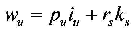
As described in Figure 7, suspension forces transmitted to the sprung mass for each axis can be expressed as follows:
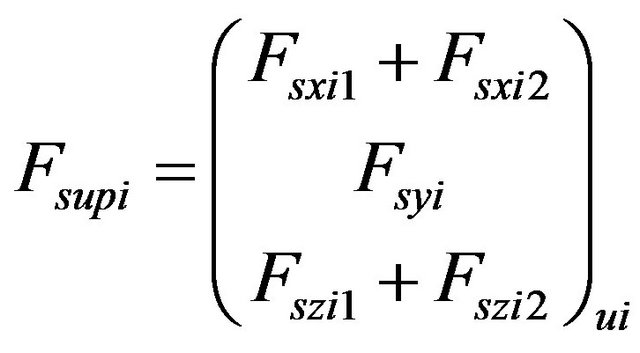 (27)
(27)
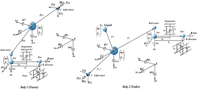
Figure 5. Vehicle mathematical model.
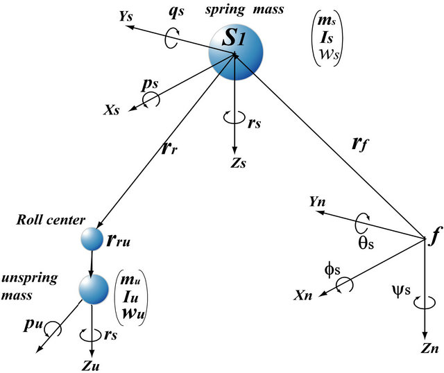
Figure 6. Unsprung mass kinematics.
where:
 and
and  are the vertical suspension forces at left and right sides respectively.
 is the internal lateral force applied to the roll center of each axis. This force is the result of the lateral forces applied to the tires.
 and
and  are the longitudinal suspension forces at the right and left sides respectively.
The suspension forces in the system attached to the sprung mass  can be defined using the transformation matrix that connects the unsprung mass and sprung mass (Equation (17)).The internal forces can be eliminated according to the dynamic equations of motion for each axis
 , as illustrated in Figure 7.
 (28)
(28)
 (29)
(29)
 (30)
(30)
2.4. Fifth Wheel Kinematics
The motion of the sprung mass of tractor and trailer are coupled via the fifth wheel joint. Several studies suggested to consider joint connection as a rigid one in the case of translational motion. This allows to consider a joint as a point. With this assumption, the number of degrees of freedom was reduced. Thus we can calculate the expressions for velocity and acceleration of the trailer
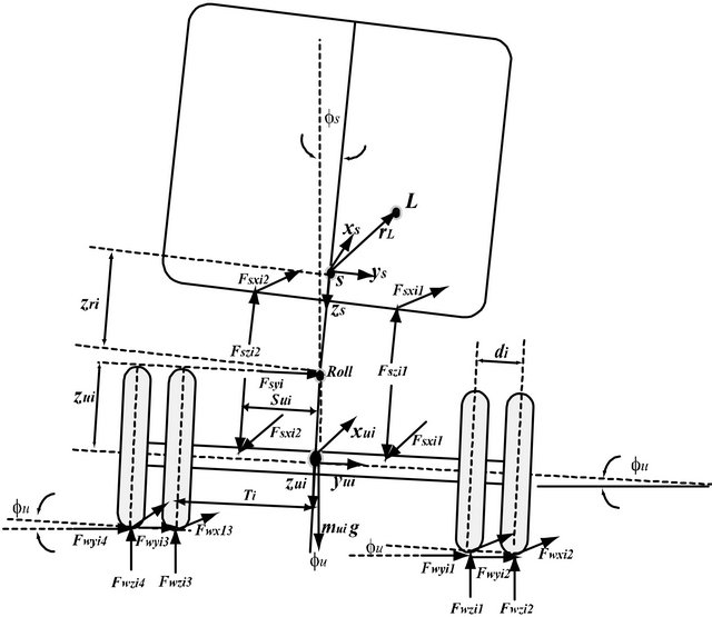
Figure 7. Vehicle model (front view).
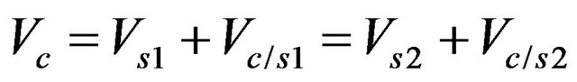
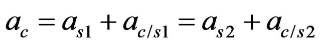
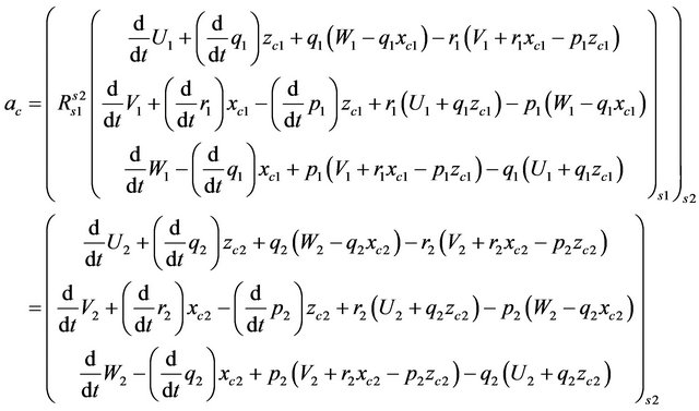
depending on the velocity and acceleration of the tractor [4]. If the harness is not rigid enough, it can be modeled as an assembly of a spring and a damper in parallel [3]. However, torsional component of the fifth wheel acts in the case of rolling motion. From Figure 8, velocity and acceleration of point C were calculated with respect to the two systems fixed to the sprung masses of tractor and trailer as follows:
 (31)
(31)
with:
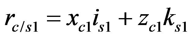 and
and 
where:
and
 (32)
(32)
The following relations can be obtained by introducing the expressions of Equation (32) in Equation (31).
 (33)
(33)
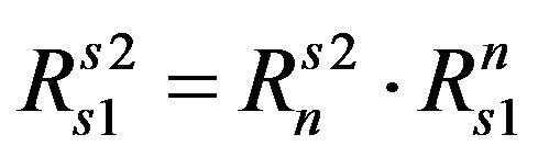
The transformation matrix  between the system attached to the sprung mass of trailer
  and the system fixed to the sprung mass of tractor
  can be calculated through the inertial system as follows:
 .
.
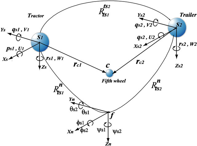
Figure 8. Fifth wheel kinematic.
 (34)
(34)
The simultaneous solution of Equations (33) and (34) gave the final expressions for the velocity and acceleration of the trailer as a function of the velocity and acceleration of the tractor.
The sweep on the roll angle between the tractor and trailer was useful to calculate the constraint of the fifth wheel for the roll motion (roll moment):
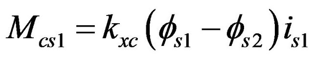
 (35)
(35)
3. Vehicle Kinetics
This section is devoted to the definition of variables with some algebraic manipulations chosen for the equations of motion. All kinetic parameters were developed for an articulated vehicle. The same settings were applied in the case of a unit vehicle. The free body diagram shown in Figure 7 shows the external and internal forces and moments applied to each subsystem of the vehicle. To obtain the equations of linear and angular motions, it is important to model the rigid body as a set of material points.
3.1. Linear Motion
The application of Newton’s laws eventually gives the equations of linear motion for the tractor and trailer.
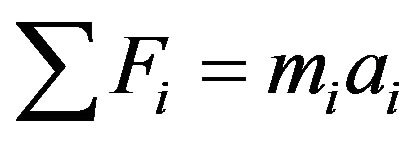 (36)
(36)
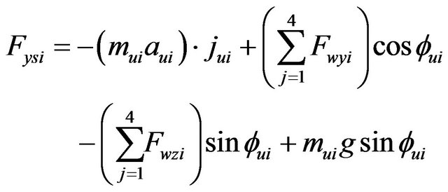
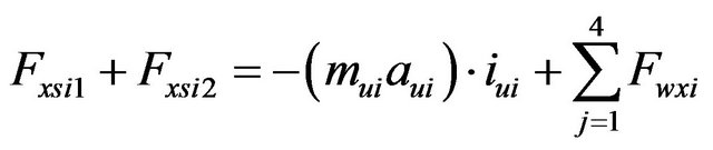
The equations of translational motion can be obtained by the combination of the Equations (36), (22), (24), (29), and (30). These equations were represented by second order differential equations for sprung mass si:

 (37)
(37)
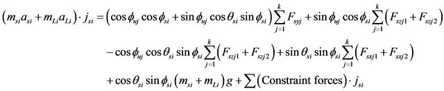

 (38)
(38)
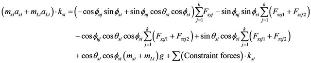 (39)
(39)
where
 : tractor
 : trailer.
 : axle number.
 : axle number.
  for tractor and
  for trailer.
 : liquid.
 : sprung mass
 .
.
In this study the constraint forces due to the fifth wheel were eliminated by using the kinematic Equations (33) and (34) developed earlier. It should be noted that all these equations of motion were programmed in the Maple software in a systematic way. Therefore, to obtain the equations of motion in the case of a unit vehicle, only change of the indices  was needed.
The equation of vertical motion of the sprung mass for each axis  was given by the folowing expression:
 (40)
(40)
where:
 : axle number.
 : number of tires in each axle.
 :
:  fortractor front axle and
  for the other axles.
3.2. Angular Motion
It is important to model the rigid body as a system of material points  with masses
  to obtain the equation of angular motion. According to Newton’s equation, angular momentum relative to the inertial system can be given by the following expression:
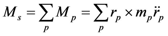 (41)
(41)
Substituting Equation (21) in (41), the following expression can be obtained:
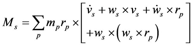 (42)
(42)
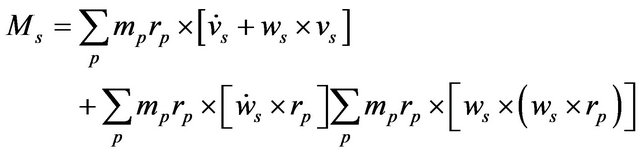 (43)
(43)
The first term of Equation (43) can be simplified as:
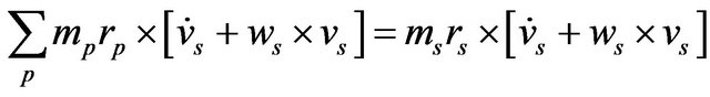
The second and third terms of Equation (43) can also be simplified [10] as:
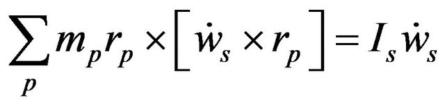
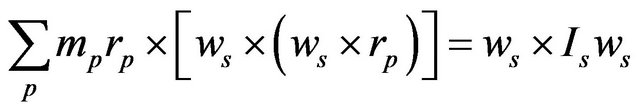
Therefore Equation (42) takes the following form:
 (44)
(44)
Since the sprung mass center coincides with the origin of the body axis system , the expression of angular motion (44) can be formulated as follows:
 (45)
(45)
The matrix of inertia  was expressed in the system
 as follows:
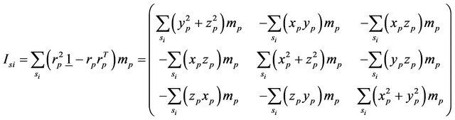 (46)
(46)
Since the tractor body and the trailer body can be modeled as contained bodies, all mathematical expressions can be expressed by integrals  instead of a sums
 .
.
The moments applied to the sprung mass due to the liquid load and the suspension forces expressed in axis system fixed to the sprung mass were calculated as follows:
 (47)
(47)
 (48)
(48)
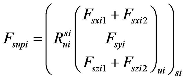
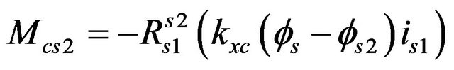
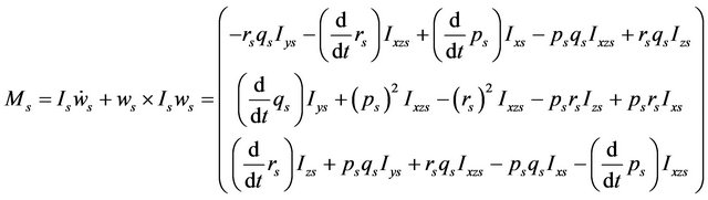
Substituting in Equation (45), the terms of the moments due to the liquid charge (47), the moments of the suspension (48) and the moments due to the fifth wheel constraints (35), the final equations of angular motion of the sprung mass (si) can be obtained as follows:


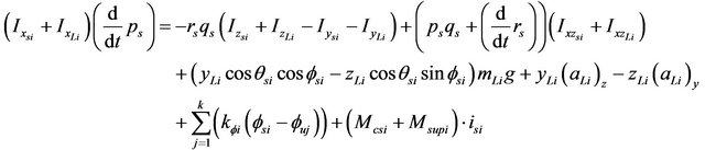 (49)
(49)
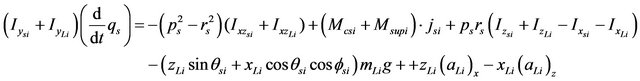 (50)
(50)
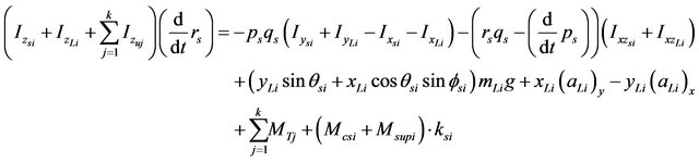 (51)
(51)
k: axle number k = 3 for tractor and k = 2 for trailer.
The equation for rolling motion of the sprung mass of each axle  can be given by the following expression:
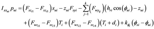 (52)
(52)
where:
 : axle index.
 : number of tires in each axle.
 :
:  for the front axle of the tractor and
  for other axles.
3.3. Suspension Model
The external forces acting on the vehicle are generated mainly due to the contact forces between wheel and ground. These forces are transmitted to the sprung mass through the suspension system of the vehicle. To simplify the model, the suspension system was represented with a linear spring and a damper assembled in parallel. The vertical force applied on the vehicle through the suspension system was assumed to be equal to the sum of the static equilibrium force and the excitation forces.
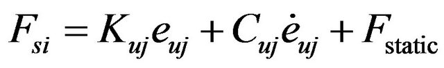 (53)
(53)
where  is the suspension deflections and can be calculated based on the geometry of the vehicle.
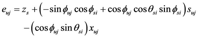
 (54)
(54)
where:
 : sprung mass of tractor.
 : sprung mass of trailer.
 : axle number (
 for tractor and
  for trailer).
3.4. Tire Model
The tire is an essential element in a vehicle. It represents the contact between wheel and ground. The forces and moments transmitted to the vehicle by the tires due to wheel-ground interaction are complex and nonlinear. These forces and moments depend primarily on normal forces, longitudinal and lateral load transfer, slip rate  and slip angles
  as illustrated in Figure 9.
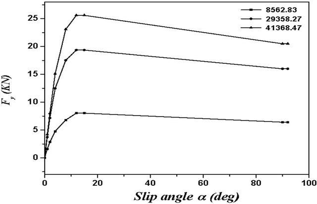
There are several models available for tires. Most studies have used linear model or models based on tables from experimental tests. The forces and moments were characterized according to vehicle velocity, normal force, longitudinal slip ratio and slip angle [4,11-14]. These models usually have a better prediction capability for the traction force of contact. However, their data are specific for the type of tire which reduces their universal use. There are other numerical models which use different analytical approaches [15-17]. The choice of model of
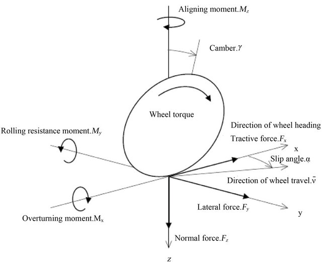
Figure 9. Forces and moments applied on the tire.
the tire affects the calculation of the efforts at the wheelsoil interface. The data from these models are important when one wants to make a dynamic model of a vehicle.
In this study the efforts of the tires were studied with the model called slip circle [11,18]. The model is closely related to the model of friction ellipse shown in Figure 10 [11].
With this model, it is possible to obtain lateral and longitudinal forces in the case of combined motions based only on measured data for separate motions such as, braking/traction alone or direction case, as illustrated in Figure 11.
The calculation was based on the evaluation of friction  and
and . The calculation of these coefficients depends on the rate of longitudinal slip
  and slip angle
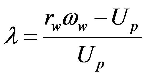
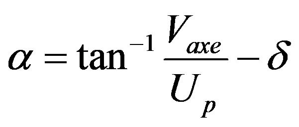
 . The rate of longitudinal slip and slip angle of the tire can be calculated by the formula:
 (55)
(55)
 (56)
(56)

where  is the radius of the wheel and
  the velocity of rotation of the wheel. Vaxe is the velocity of lateral translation of the axis and Up is the longitudinal velocity of the tire as shown in Figure 12.
The expressions can be evaluated from the velocity of center of mass of the vehicle.
 (57)
(57)
 (58a)
(58a)
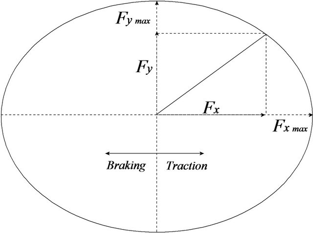
Figure 10. Friction ellipse concept.
 (a)
(a)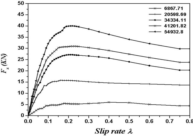 (b)
(b)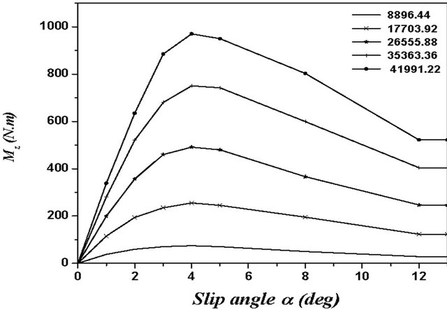 (c)
(c)
Figure 11. (a) Lateral tire-road contact force; (b) Longitudinal tire-road contact force; (c) Aligning moment generated at tire-road contact. Experimental forces and moments generated at tire-road contact for several vertical load charge [19].
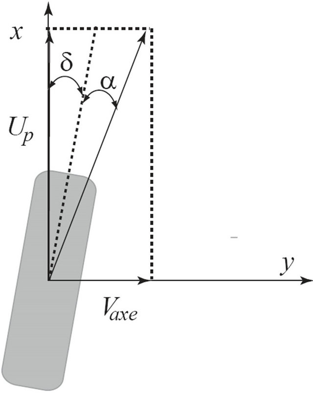
Figure 12. Tire model.
 (58b)
(58b)
3.4.1. Tire Vertical Load
In this study, the vertical load of the tire was modeled as a linear spring. Therefore, the vertical force depended on the spring constant.
 (59)
(59)
The tire deflections were calculated from the geometry of the vehicle as follows:
 (60)
(60)
 (61)
(61)
To calculate the combined forces, a dimensional vector of slip amplitude  and direction
  was defined [20] as:
 (62)
(62)
The coefficients of friction between the tire and the ground, in the case of the combined forces, took the forms below:

 (63)
(63)
Finally, longitudinal and lateral forces in the case of combined motion were calculated:
 (64)
(64)
3.4.2. Braking Force
The braking force was calculated by taking into account forces and moments developed in the wheel due to rotation (spin) of the wheel as shown in Figure 13. Acceleration of rotation (spin) of the wheels  were calculated from the rotational motion of the wheels as follows [21]:
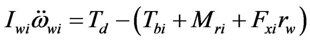 (65)
(65)
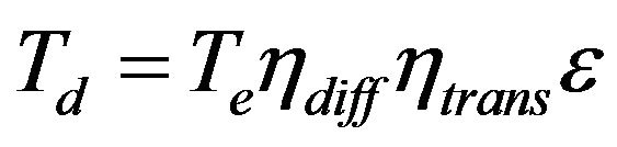
Figure 13. Wheel dynamics.
4. Vehicle Model Validation
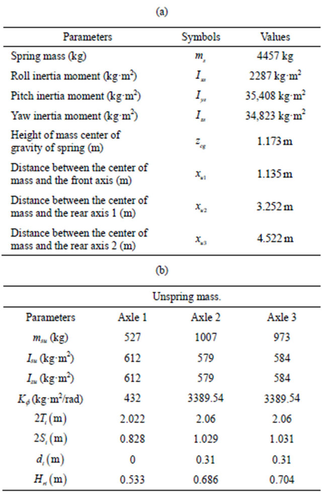
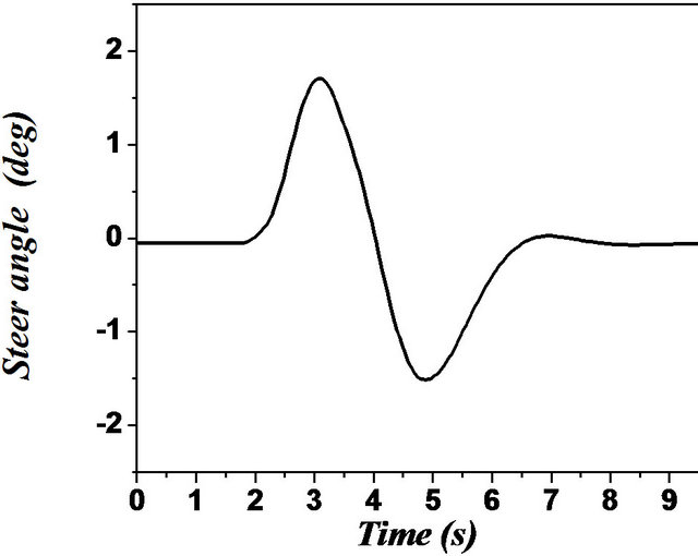
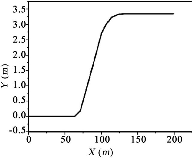
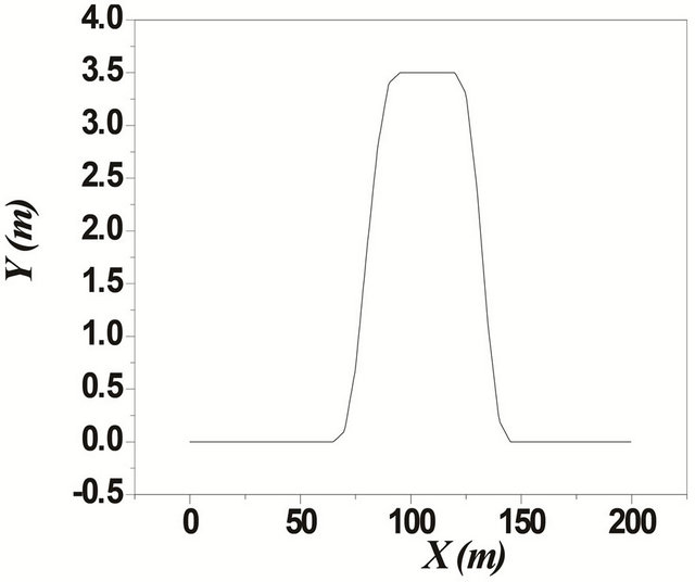
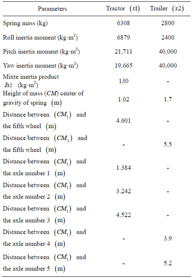
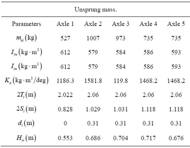
The TruckSim software, developed by the transportation center of the University of Michigan (UMTRI), is specialized in the simulation of heavy vehicles [15,19,22]. The center also developed software applications: CarSim for tourist vehicles and BikeSim for motorcycles. TruckSim, the most popular software in this field, was used to represent and study the dynamics of vehicles in a computer environment. It is possible to analyze a large number of vehicle configurations, since the software has a library of existing models in the transportation industry. However, TruckSim can only add a load that is considered to be fixed on the semi-trailer. This feature does not allow to study the dynamic behavior of liquid sloshing in tanker trucks. The TruckSim library also has a number of predefined trajectories and maneuvers that can enable researchers to validate the behavior of the vehicle model developed, for difficult maneuvers such as motion in a curve, change of single and double lanes. In the TruckSim environment, the maneuvers are predefined paths, i.e., the excitation is represented by a displacement vector. However, for the model developed in this study, the excitation was defined by the angle of steering or braking torque as an input parameter. From the output vector, the response of the steering angle was recorded. This response was the input parameter for our model that considered the same configuration for a unit or articulated vehicle as defined by the Tables 1 and 2 in the annexure [22]. Two lane change maneuvers (single and double) with a constant speed  were chosen to compare the two models. Figure 14 shows the trajectory and the steer angle during the two maneuvers [22].
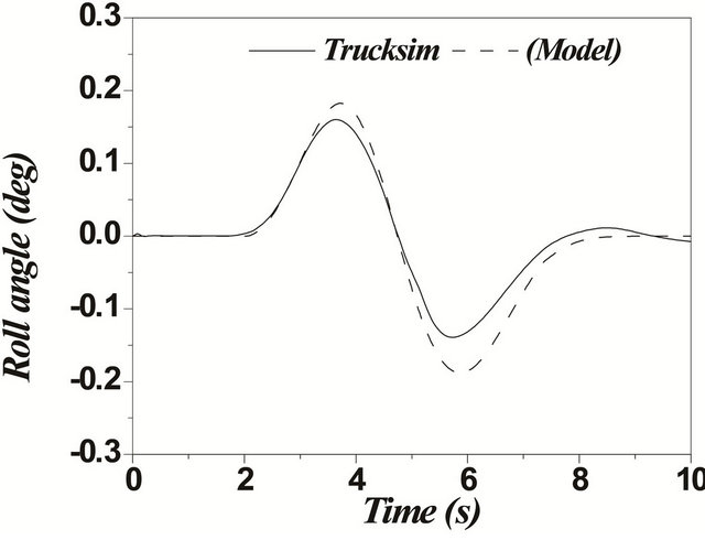
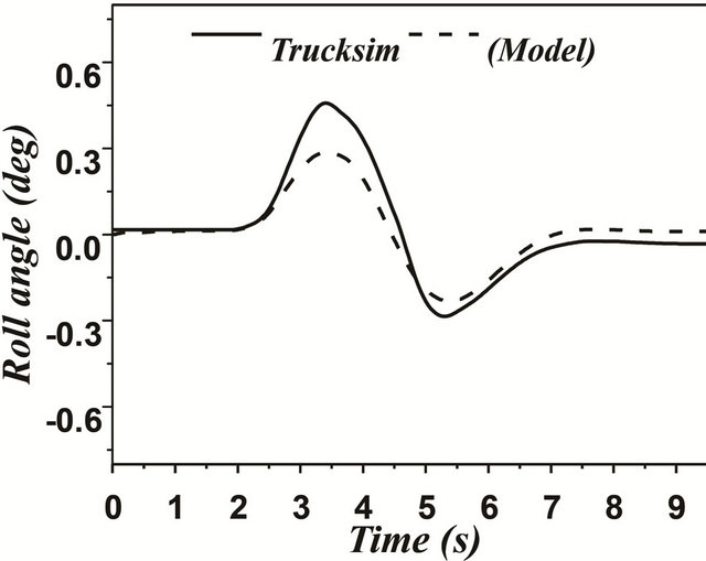
Figures 15 and 16 represent the comparison between model simulations for the unit vehicle and the TruckSim software respectively. The vehicle directional responses were evaluated using two difficult motions, such as change of single and double lanes. This comparison was characterized in terms of roll angle, lateral acceleration of the center of mass and trajectory traveled from the center of mass. The simulation showed a good correla
Table 1. Geometric parameters of unit vehicle.
 (a)
(a) 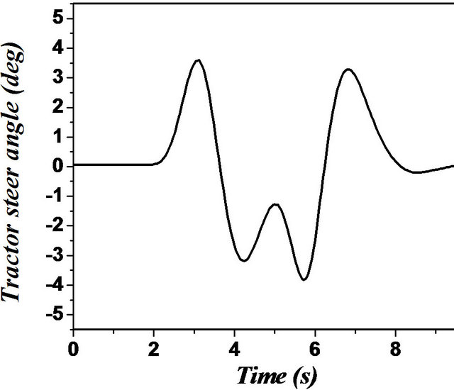
 (b)
(b)
Figure 14. (a) Simple lane change maneuver and the desired trajectory; (b) Double lane change maneuver and the desired trajectory. Maneuvrer used for the comparaison between the model and TruckSim software.
Table 2. Geometric parameters of articulated vehicle.
(a)
(b)
tion between the two models. A small difference was noted for the trajectory of the center of mass. This difference may be due to the steering angle error of the output vector obtained using TruckSim. In addition, excitement used for the TruckSim software was in closed loop (predefined trajectory).
 (a)
(a)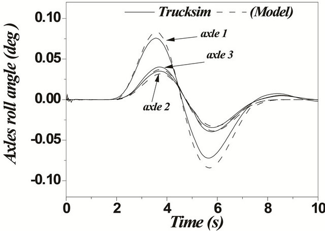 (b)
(b)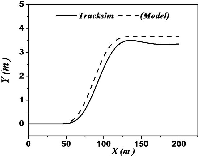 (c)
(c)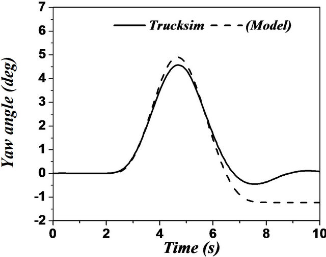 (d)
(d)
Figure 15. (a)-(d) Single lane change maneuver for a unit vehicle (Solid: trucksim; Dashed: model).
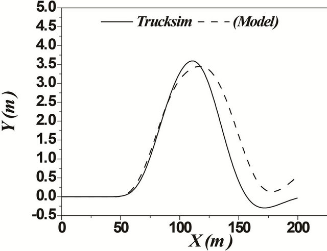
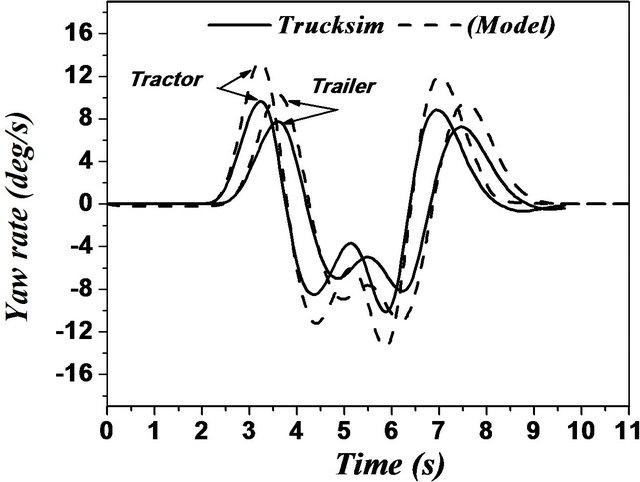
In case of articulated vehicles, the analysis was more complicated. This difficulty was due to addition of the hinge point where there were additional forces and moments acting between the tractor and trailer. Figures 17 and 18 represent the comparison between the two models for the same difficult issues such as motions during change of single and double lanes. A good overall correlation was observed. However, our model underestimated the response to some extent. This difference in response was observed due to yaw motion. TruckSim software
 (a)
(a)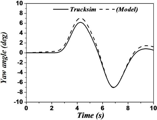 (b)
(b)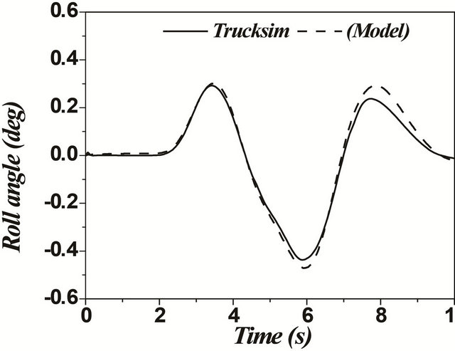 (c)
(c)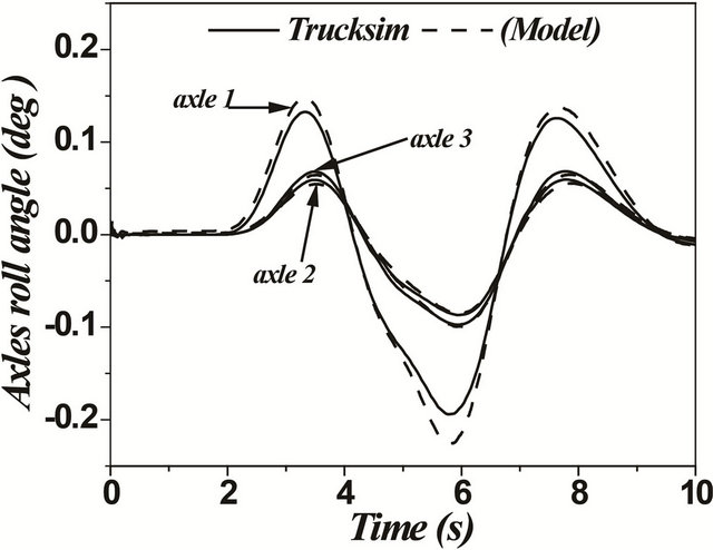 (d)
(d)
Figure 16. (a)-(d) Double lane change maneuver for a unit vehicle (Solid: trucksim; Dashed: model).
was able to handle such situation in a better way. This difference can be explained based on the assumption that the fifth wheel was considered as a rigid body for our model. However, in TruckSim it was modeled by a spring-damper combination, which can represent multibody connections between subsystems in a better way. The increase in the response of yaw motion influenced
 (a)
(a)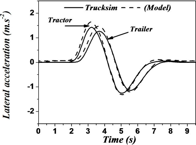 (b)
(b)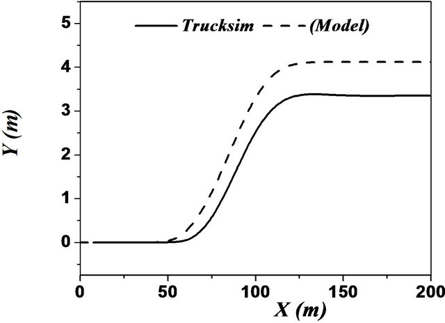 (c)
(c)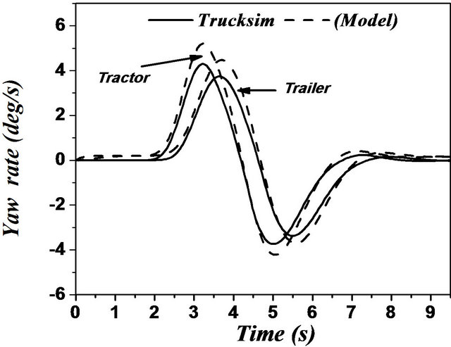 (d)
(d)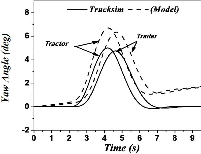 (e)
(e)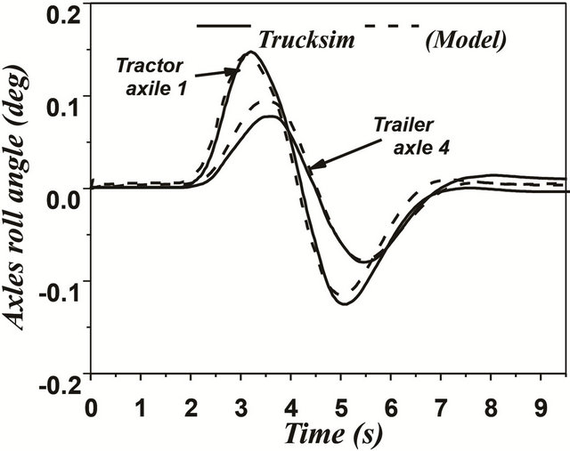 (f)
(f)
Figure 17. (a)-(f) Single lane change maneuver for an articulated vehicle (Solid: trucksim; Dashed: model).
 (a)
(a)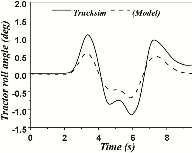 (b)
(b)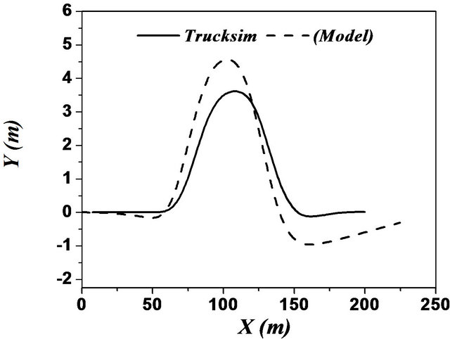 (c)
(c)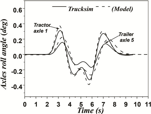 (d)
(d)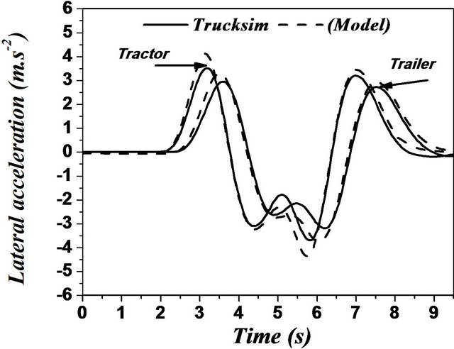 (e)
(e)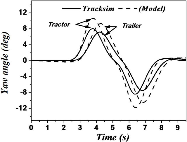 (f)
(f)
Figure 18. (a)-(f) Double lane change maneuver for an articulated vehicle (Solid: trucksim; Dashed: model).
the trajectory of the vehicle as illustrated by Figures 17 and 18. This may be due to the error of steering angle recorded from the TruckSim output vector. Still, this difference did not practically affect the very good corre lation between the two models.
5. Conclusions
A complete nonlinear three-dimensional vehicle model was developed and validated by Trucksim software. Both unit vehicle and articulated vehicle combination systems were considered in this study. The model gave realistic results in simulation of handling maneuvers near and beyond the adhesion limits.
The loadtransfer for mobile charge due to the liquid was accurately modeled and integrated into the vehicle model as a multibody system. The dynamic responses of tank vehicles were further investigated in view of variations in vehicle maneuvers, fill volume, road condition, and tank configuration [8].
This research, can help better understanding of this kind of complex problem. This will make it possible to answer some queries in the field of safety and the stability of the heavy vehicles, in particular for the tanktruck.
REFERENCES
- J. Ellis, “Vehicle Handling Dynamics,” Mechanical Engineering Publicantions, London, 1994.
- H. Dongyoon, “Predictive Modeling and Active Control of Rollover in Heavy Vehicles,” Ph.D. Dissertation, Texas University, Austin, 2001.
- C. B. Winkler, J. E. Bernard and P. S. Fancher, “A Computer Based Mathematical Method for Predicting the Directional Response of Truck and Tractor-Trailers,” Technical Report, Highway Safety Research Institute, University of Michigan, Ann Arbor, 1973.
- A. Ann, R. D. Ervin and Y. Guy, “The Influence of Weights and Dimensions on the Stability and Control of Heavy-Duty Trucks in Canada,” Volume III Appendices, Final Report, Vehicle Weights and Dimensions Study 2, University of Michigan, Transportation Research Institute, 1986.
- M. Sayers, “Symbolic Computer Methods to Automatically Formulate Vehicle Simulations Codes,” Ph.D. Dissertation, University of Michigan, Ann Arbor, 1990.
- M. Toumi, M. Bouazara and M. J. Richard, “Analytical and Numerical Analysis of the Liquid Longitudinal Sloshing Impact on a Partially Filled Tank-Vehicle with and without Baffles,” International Journal of Vehicle System Modeling and Testing, Vol. 3, No. 3, 2009, pp. 229-249. doi:10.1504/IJVSMT.2008.023840
- M. Toumi, M. Bouazara and M. J. Richard, “Impact of Liquid Sloshing on the Behavior of Vehicles Carrying Liquid Cargo,” European Journal of Mechanical Engineering/Solids, Vol. 28, No. 5, 2009, pp. 1026-1034.
- M. Toumi, “Études et Analyse de la Stabilité de Camions Citernes,” Ph.D. Dissertation, University of Quebec at Chicoutimi, Canada, 2008, 178 p.
- Maple 9. http://www.maplesoft.com/
- K. Meriam, “Engineering Mechanics,” 5th Edition, Vol. 2, Wiley, Hoboken, 2002.
- H. B. Pacejka, “Tire and Vehicle Dynamics,” 2nd Edition, 2005.
- H. Pacejka and E. Bakker, “The Magic Formula TyreModel,” Proceedings of 1st International Colloquium on Tyre Models for Vehicle Dynamics Analysis, 1991, pp 1-18.
- J. Y. Wong, “Theory of Ground Vehicles,” 3rd Edition, John Wiley and Sons, Hoboken, 2001.
- U. Kiencke and L. Nielsen, “Automotive Control System,” Springer, Berlin, 2000.
- F. Ben Amar, “Modèle de Comportement des Véhicules Tout Terrain pour la Planification Physico-Géométrique des Trajectoires,” Ph.D. Dissertation, Université Pierre et Marie Curie, France, 1994.
- J. Svendenius and M. Gafvert, “A Semi-Empirical Dynamic Tire Model for Combined-Slip Forces,” Vehicle System Dynamics, Vol. 44, No. 2, 2004, pp. 189-208.
- M. Gafvert, J. Svendenius and J. Andreasson, “Implementation and Application of a Semi-Empirical TireModel in Multi-Body Simulation of Vehicle Handling,” Proceedings of the 8th International Symposium on Advanced Vehicle Control, Taipei, 2006.
- W. Pelz, D. Schuring and M. G. Pottinger, “A Model for Combined Tire Cornering and Braking Forces,” SAE Paper, 960180, 1996.
- M. W. Sayers and S. M. Riley, “Modeling Assumptions for Realistic Multibody Simulations of the Yaw and Roll Behavior of Heavy Trucks,” SAE Paper, 960173, 1996.
- M. Sanfridson, M. Gafvert and V. Claesson, “Truck Model for Yaw Dynamics Control,” Technical Report, Lund Institute of Technology, Sweden, 2000.
- D. Syndey, D. Terry and G. Roberts, “A New Vehicle Simulation Model for Vehicle Design and Safety Research,” SAE, Engineering Dynamics Corp., (2001)-01- 0503.
- Truckism 6. http://www.carsim.com/
Definitions of Symbols
 : Longitudinal velocity of sprung mass
 ;
;
 : Lateral velocity of the sprung mass
 ;
;
 : Yaw rate of the sprung mass
 ;
;
 : Roll rate of the sprung mass
 ;
;
 : Distance between the two tires;
 : Distance between the center of mass of the axle
  and the center of (one tire or dual tires);
 : Longitudinal distance between the center of mass of the axle
  and the center of the sprung mass
 ;
;
 : Vertical distance between the roll center of the axle
  and the center of the sprung mass
 ;
;
 : Vertical distance between the roll center roll of the axle
  and the road;
 : Initial deflection due to static deflection;
 : Sprung mass vertical displacement
 ;
;
 : The vertical distance between the roll center and center of the axle
 ;
;
 : Initial vertical distance between roll center and center of the axle
 ;
;
 : The vertical distance between the roll center and center of mass of the sprung mass
 ;
;
 : Moment due to constraints of the fifth wheel;
 : Moment due to the suspension forces;
 : Wheel drive troque;
 : Engine torque;
 : Wheel braking torque;
 : Wheel moment of inertia;
 : Transmission ratio;
 : Différentiel ratio;
 : Torque function (the fraction of engine torque applied to the specific wheel);
 : Longitudinal tire-road contact force;
 : Resistance moment of the tire.
NOTES
*Corresponding author.