World Journal of Mechanics
Vol. 1 No. 4 (2011) , Article ID: 7128 , 6 pages DOI:10.4236/wjm.2011.14025
Transverse Standing Waves in a Nonuniform Line and Their Empirical Verifications
University College, Pennsylvania State University, York, USA
E-mail: has2@psu.edu
Received May 23, 2011; revised June 19, 2011; accepted July 1, 2011
Keywords: Nonuniform line, Standing waves, Airy functions, Mathematica
ABSTRACT
We consider a one-dimensional elastic line with a linear varying density. Utilizing a Computer Algebra System (CAS), such as Mathematica symbolically we solve the equation describing progressive transverse waves yielding standing waves. For a set of suitable parameters the numeric mode of Mathematica displays and animates vibrating normal modes bringing the vibrations to life. We tailor a device that mimics the characteristics of the non-linearity; experimentally we explore its integrity.
1. Introduction and Motivation
The description of progressive transverse and longitudinal waves in a uniform non-dispersive elastic media is trivial. This is discussed in introductory physics and engineering undergraduate college textbooks [1-3]. Despite being trivial they are useful and practical describing the characteristics of waves occurring in nature such as water waves, light waves, and sound waves, and in manmade media such as string waves and etc. In its simplest scenario, in one-dimension, combining two identical traveling waves progressing in opposite directions results in standing waves. Meaning, given the appropriate parameters the superposition of the waves may result in constructive and destructive interferences making the displacement of the elastic media maximum or zero, respectively. The uniformity of the media yields spreading evenly the nodal and anti-nodal points along the line. The vibrating media with specific vibrating frequencies appears as if it were standing still. The normal modes of these standing waves are distinguished with their frequencies; frequencies of the higher excited modes are integer multiples of the frequencies of the lower normal modes. In other words, frequencies of the harmonics are related via integer multipliers.
For a nonuniform non-dispersive media the scenario is quite different. Envisioning designing an experiment that mimics the characteristics of a nonlinear media in our current search we focus on analyzing the characteristics of transverse standing waves. As we discuss in Section 2, the fundamental difference between a uniform vs. a nonuniform elastic media is the impact of the latter on the traveling waves. The equation describing the former in one-dimension is trivial and is solved at ease [1-3]. On the other hand for the latter, solving the equation and implementing the boundary conditions conducive to the standing waves mathematically is challenging. In general, deviating from a monotonically increasing density results in mathematical challenges; some of the issues are addressed in the Conclusions section.
A thorough literature search reveals that there are a limited number of research articles that have discussed the traveling waves in nonlinear media; [see references within 4]. In our view [4] is a comprehensive article. Aside from being analytical the author with much effort composed a cumbersome computer code deducing the needed numeric values; however, the author displayed only one normal vibrating mode. With the advent of a Computer Algebra System (CAS), such as Mathematica [5] we investigate similar issues bringing to the forefront a host of fresh generalizations. From the author's point of view solving the needed ODE utilizing Mathematica is as powerful as solving the same equation the traditional way. The payoff is the time saved shortening the analytic formulation then invested in exploring fresh ideas, such as devising complementary experiment for a better understanding. Moreover, the augmented numeric analysis is conducive not only displaying normal modes, but also animating the associated standing waves, features that forcefully were left out in the pre-CAS era. With these objectives we craft this note as follows. In addition to Introduction and Motivation, in Section 2, The Physics of the Problem, we lay down the foundation of the needed fundamentals. In Section 3, Analysis, applying Mathematica we solve the time independent piece of the wave equation analytically. In this section for a set of suitable parameters we evaluate the numeric values of the functions displaying the normal modes of the vibrations. In Section 4, Experiment, we discuss the characteristics of the manufactured replica. Utilizing data we correlate our analysis to the non-linearity of the line. We close our search making a few conclusive remarks suggesting how to generalize the features of our study.
2. The Physics of the Problem
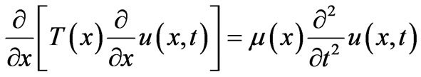
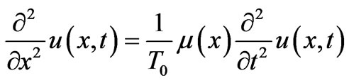
It is known that the wave equation for displacement of a uniform string from its equilibrium position is given by [2, and reference 3 within],
 (1)
(1)
where u(x,t) is the displacement, T(x), and μ(x) are the position dependent tension and density of the line, respectively. Assuming the latter two quantities are constants, i.e. T(x) = T0 and , (1) assumes the classic form,
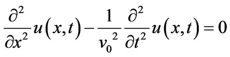 (2)
(2)
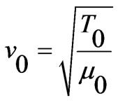
where the speed of the traveling signal is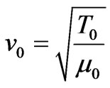
 .
.
Equation (2) has a separable solution, namely,
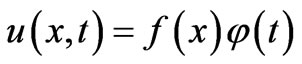 with
with 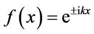 and
and 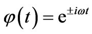
 such that
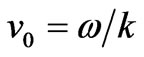 . Equation (2) yields,
 (3)
(3)
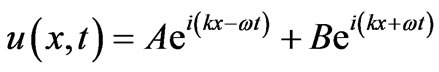
Meaning, (1) being a linear ODE yields the superposition of the individual solutions. These are interpreted as being progressive signals along the stretched line. The first term describes a wave traveling from left to right and the second term is the description of a wave progressing from right to left, respectively. This can also be written as sinusoidal functions such as,
 .
.
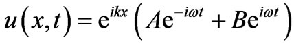
The latter is the standard notation typically used in introductory text books. The advantage of writing the solution according to (3) vs. the alternate  is that the former can be written as,
 (4)
(4)
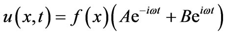
The factored function  is the sinusoidal position dependent term of the traveling wave. This simple function inherits the homogeneity characteristics (constant density) of the line. For an inhomogeneous line, however, (4) may be generalized. Meaning, assuming constant tension, (1) reads,
 (5)
(5)
The time dependence of (5) is the same as (1). Therefore, their associated time dependent solutions are the same as well. On the other hand, the coordinate dependent solution of (5) is f(x), such that,
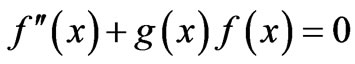 (6)
(6)
where g(x) is an x-dependent function. Among other things it embraces the inhomogeneity of the line; we share more on this in the next paragraph. Hence, the formal solution of (5) is,
 (7)
(7)
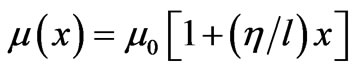
For a nonuniform line we consider the same coordinate dependent function as [4], namely,
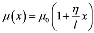 .
.
The  is the x-dependent density of the line; its density increases monotonically from one end to the other end of the length
 . Parameter
  according to
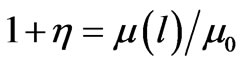 is the ratio of the densities evaluated at both ends; is the corresponding density of a uniform line. Accordingly g(x) reads,
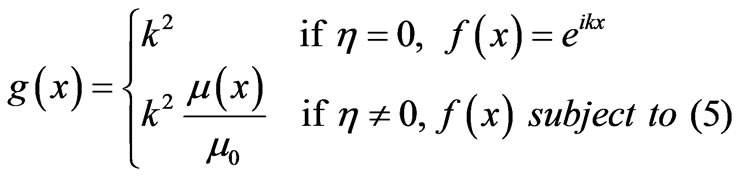 (8)
(8)
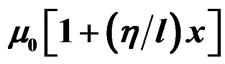
We have also considered a variety of functions such as quadratic density function,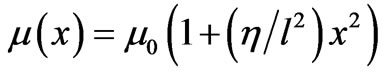 . We made comments concerning this function in the Conclusions section.
3. Analysis
The task at hand is to evaluate . The code solving (6) utilizing Mathematica for
  given by (8) is,
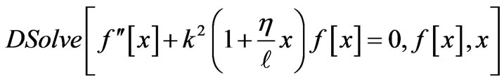
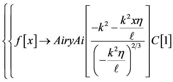
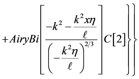
The solution is a linear combination of two distinct Airy functions. The AiryAi and AiryBi are the first and the second kind of Mathematica library Airy functions, respectively. The coefficients C[1] and C[2] are to be determined by applying the desired boundary conditions. For instance clamping both ends of the line imposes . These boundary conditions yield a set of two linear independent equations. The nonzero solution of the latter requires a null Wronskian, i.e. W = 0. The solution of the latter calls for a numeric computation. For a set of numeric parameters corresponding to the physical properties of the line such as, length
  and density parameter
  we seek for value (s) of k subject to W = 0. Considering the fact that all four elements of the
  Wronskian are oscillatory Airy functions deducing successfully numeric values for k from such a challenging equation brings a great deal of appreciation to the superb computational power of Mathematica. The abscissas of the intercepts of the Wronskian with the horizontal axis as shown in Figure 1 are the roots of W = 0. The Mathematica code yielding Figure 1 is a modified version of the code [6].
By varying the value of  and repeating the procedure conducive to Figure 1, we tabulate the results in Table 1; this is the extended and more accurate version of Table 1 [4].
The tabular values of  according to Table 1 clearly show the impact of the in homogeneity of the line. The heading of the first column, n, is the indicator of the
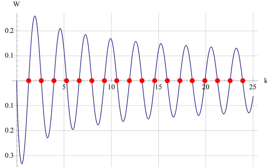
{{k®1.2643},{k®2.60158},{k®3.93683},{k®5.2704},{k®6.60282},{k®7.93443},{k®9.26543},{k®10.596},{k®11.9262},{k®13.2561},{k®14.5857},{k®15.9152},{k®17.2445},{k®18.5737},{k®19.9028},{k®21.2318},{k®22.5607},{k®23.8895}}
Figure 1. Plot of W vs. k for h = 10.0. The list is the coordinates of the abscissa shown by the dots.
number of the nodal points between the two clamped ends of the line. E.g. n = 0 corresponds to no nodes and n = 7 means seven nodes. The second column with equally spaced  is indicative of harmonic vibrations. The remaining headings are the values of the in homogeneity given by parameter
 . The numbers underneath each corresponding
  are to be compared to the associated values of the harmonic waves, i.e. the second column. One observes for instance for a chosen
  the “wavelengths” are variable. For the sake of comprehension Figure 2 shows the first six normal vibrating modes of a homogeneous line vs. the corresponding inhomogeneous line for
  = 10.0.
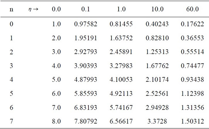
Table 1. Extended Table 1 [4]. The first column is the number of the nodes, n. The headings of the remaining columns are the values of h. The tabulated numbers are the values of k/π.
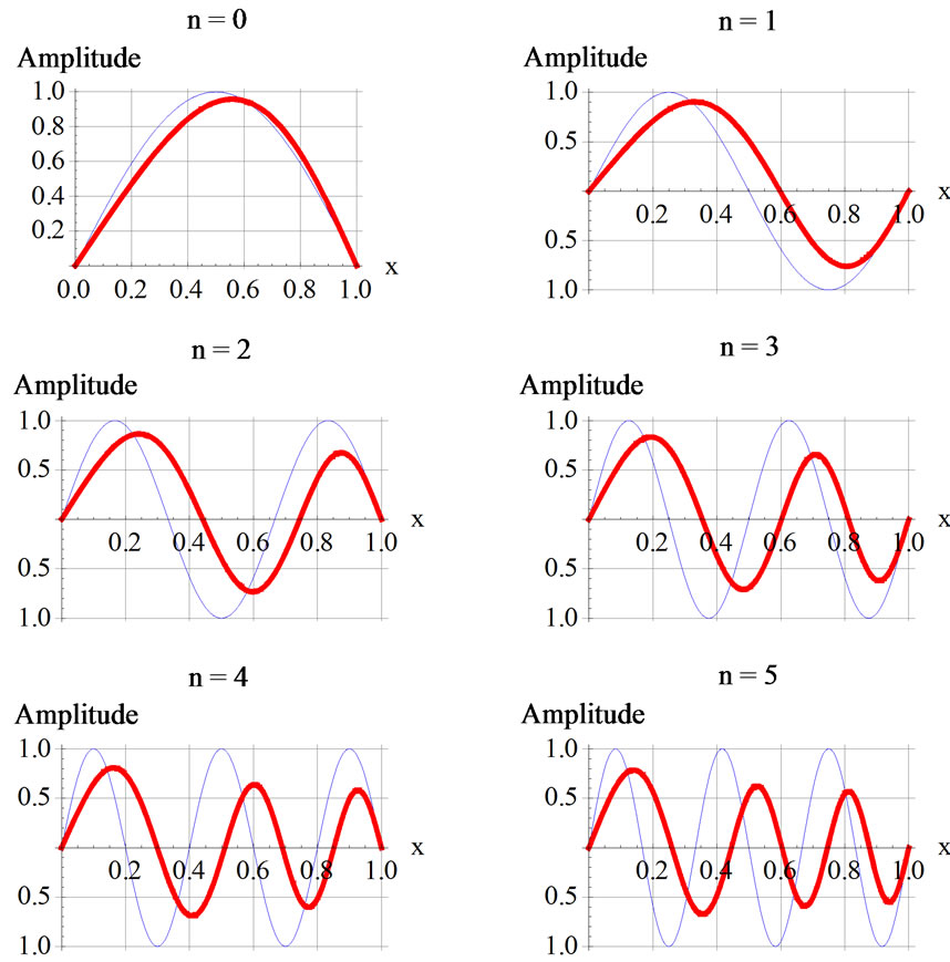
Figure 2. Display of the first six normal vibrating modes of a uniform (h = 0, the blue curves) and the nonuniform (h = 10.0, the red curves) line.
In Figure 2 for the sake of clarity the amplitudes of the nonuniform line (the red curves) are multiplied by a factor 3. The plot labels (nodal indices) in these graphs are the same as the ones used in Table 1. One observes that for the uniform line (the blue curves) the vibrations are cyclic, i.e. throughout the entire length of the line the wavelengths stay the same and the amplitudes within them are the same from one segment to the adjacent segment. On the contrary, for the nonuniform line (the red curves) the wavelengths are not the same. In fact while approaching from the light to the heavy end (from left to right) the wavelengths are shortening and the amplitudes within them as shown systematically are diminishing.
With this wealth of information in hand, one may animate the vibrations bringing the standing waves to life. E.g. Figure 3 is a snapshot of the animation of the fifth mode for an inhomogeneous  = 10.0 line.
4. Experiment
One of the objectives of our investigation is to seek a real-life setting supporting the characteristics of the proposed idealized theoretical phenomenon. The challenge is to design/tailor a device that mimics the properties of a monotonically increasing density of a one-dimensional line. In principal it is plausible to manufacture one such replica; instead, the author considered a planar isosceles triangular homogeneous strip that replicates the same general characteristics. The verification of the design is explained in detail in the next paragraph. Assuming the proposed model is just, the ancillary issue is to verify whether the one-dimensional classic standing wave formulation is applicable to a two-dimension vibrating media; we rectify this issue first.
The frequencies of one-dimensional standing waves with progressive wave speed
 is
is 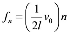 [1-3,9].
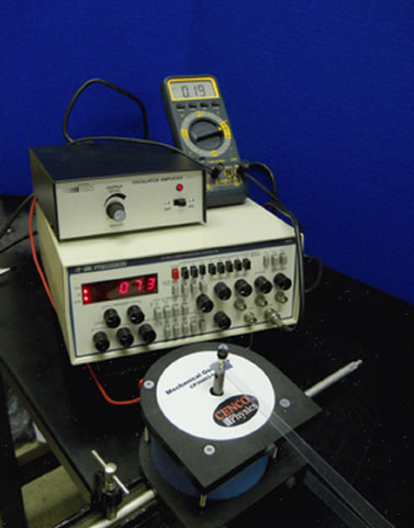
Our experiment set-up is shown in Figure 4. Accordingly, T0 = hanging weight = Mg and  = density of the homogeneous line =
 .
.
This yields, 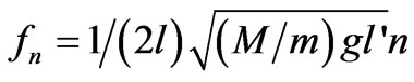 where
where  is the length of the vibrating piece and
  is the entire length. The experiment set-up is composed of a Mechanical Oscillator (the blue unit in the foreground) [7a], a Function Generator (the white unit with a digital display panel) [7b], an Oscillator Amplifier (the white unit sitting on the Function Generator) [7c], and an Ammeter (the blue rectangular unit adjacent to the Amplifier) [7d]. The vibrating elastic media is a rectangular plastic strip [8]; it is a 86.36 cm × 1.3 cm rectangle. It is mounted horizontally with its one end fastened to the oscillator and its other end running over a horizontal brass rod being pulled with a hanging weight. For our experiment incorporating the accuracy of the measured quantities, such as the masses, gravity constant, and lengths, yields to a 0.6% systematic error, i.e. fn = fn ± 0.6%.
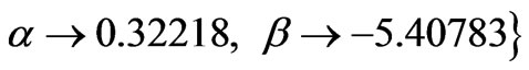
It is the objective of this phase of our experiment to verify whether this one-dimensional formulation is just for the two-dimensional rectangular strip. Applying the above formulation to the rectangle the predicated frequencies along with the systematic errors are tabulated in Table 2. The table contains the associated measured frequencies as well.
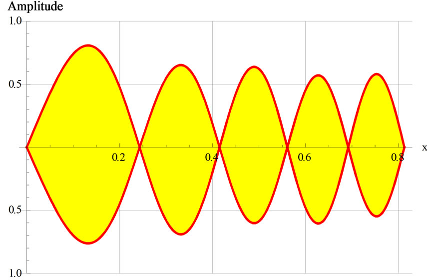
Figure 3. Fifth normal mode of the standing wave of an inhomogeneous line with inhomogeneity parameter h = 10.0.
 (a)
(a)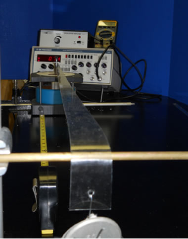 (b)
(b)
Figure 4. The left photo (a) is the photo of the hardware, the right photo (b) is the actual experiment set-up.
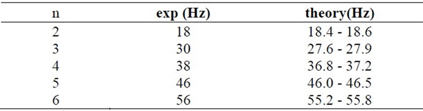
Table 2. The first column is the number of the loops, the second and the third columns are the data and the corresponding range of theoretical frequencies, respectively.
An experienced reader who worked in physics labs and who is familiar with the “standing wave experiment in a homogeneous line”[9] would agree that judging the formation of perfect standing waves are subjective; the same applies to a two-dimensional strip. Hence, the measured frequencies entered in the second column of Table 2 should not be considered as absolute. Therefore, with this notion according to Table 2 there is a reasonable agreement between the data and the theory. Accordingly, we conclude that the fundamental frequency equation given in the previous paragraph is applicable to a twodimensional homogeneous strip.
Now we move on to the two-dimensional model replica. Figure 5 depicts a homogeneous isosceles triangle with the height and base length of l and 2h, respectively. Its center of mass (c.m.) is along the x-axis and is
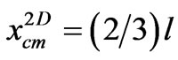 . On the other hand for a 1D line with monotonically increasing density,
the coordinate of the c.m. is
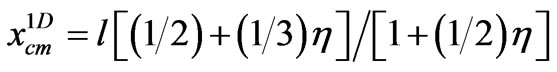 .
.
For large values of  these two coincide. That is to say a 2D homogeneous isosceles triangle acts as a 1D inhomogeneous line provided the in homogeneity parameter is “large”. The largeness of the latter is subjective; we look more on this topic in the next paragraph.
The drawing in Figure 5 is to be compared to the actual strip used in the experiment; see photo 4b. To continue with our experiment, we replace the rectangular strip with the isosceles triangular one. The measured frequencies of the associated standing waves are tabulated in Table 3.
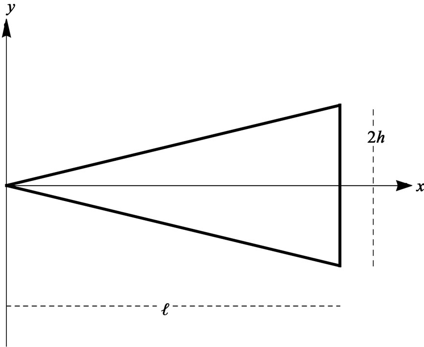
Figure 5. Display of a homogeneous isosceles triangular plastic strip.
With our set-up we were able distinctly observe the first three standing waves with corresponding three, four and five loops. By comparing Tables 2 and 3 one realizes their common features; e.g. the higher the number of loops the higher the frequencies. However, the measured frequencies tabulated in these two tables are considerably different.
Now the question is “What are the appropriate values of the ?” To answer this question we propose a semiempirical approach. It is plausible to assume the speed of the progressive waves for the rectangular and the triangular strips are the same; this is because they are cut out from the same plastic sheet and have almost comparable dimensions. The frequency of the n-th mode for the uniform rectangle is
 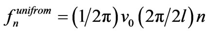 and for the nonuniform triangular strip is
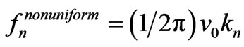 . Dividing these two equations yields
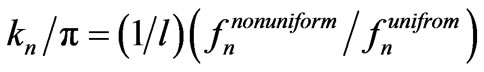 .
.
For the chosen n utilizing the measured frequencies of Table 2 and 3, we evaluate the corresponding value of kn. Then we solve (6) and search for the  conducive to the same value of
 ; in practice this requires patience! Results are tabulated in Table 4.
According to Table 4 different normal standing modes require different inhomogeneity parameter ; this was observed [4]. Utilizing Table 4 we search for
  (n). The search yields,
 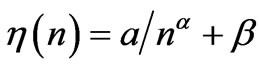 with
with 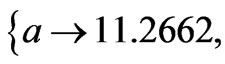
 i.e. with our approach we have established a semi-empirical analytic relationship between the in homogeneity parameter
  and the number of loops. This has been observed, however the method is different [4]. Now we take a step backward and visit the issue “How viable is our proposed triangular isosceles model replica?” Let’s remind ourselves that a perfect model requires a “large”
 . Our evaluated
 ’s are tabulated in Table 4. Figure 6 shows the deviation of the characteristics of the proposed model replica vs. a perfect case.
In Figure 6 the dot on each line is the coordinate of the c.m. for  = 1.3, 1.5 and 2.5, respectively. The black vertical line is the position of the c.m. for
 “
“ ”. The Gray vertical line is the position of the c.m.
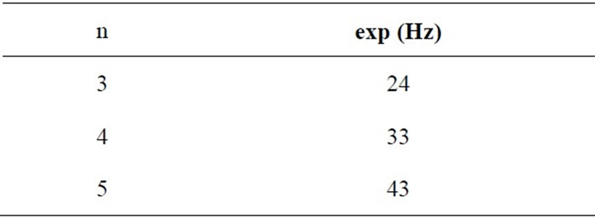
Table 3. The first column is the number of the loops of the standing waves and the second column is its associated measured frequencies.
Table 4. The first column is the number of the loops of the standing waves; the second column is its associated inhomogeneity parameter h.
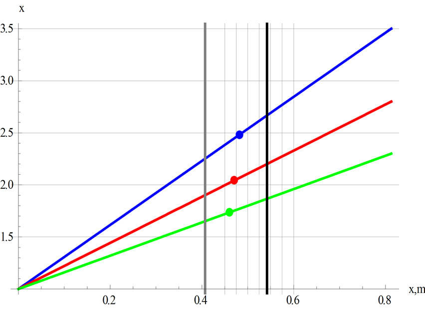
Figure 6. The solid slanted lines are the plots of 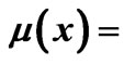
 for
for  = 1.0,
  = 0.81 m and h = 1.3, 1.5 and 2.5 corresponding to green, red and blue, respectively.
for a uniform one-dimensional line. Accordingly, the accuracy of our proposed two-dimensional replica is within 11% to 15%, corresponding to  values 2.5 to 1.3, respectively.
5. Conclusions
The author had two major objectives tackling the proposed problem. 1) Utilizing a Computer Algebra System (CAS) such as Mathematica to analyze symbolically and numerically the various aspects of the progressive waves conducive to standing waves in an inhomogeneous line. 2) Devise an experiment verifying the feasibility of the proposed theoretical analysis in a real-life setting. Concerning the first objective throughout the article it is shown how the traditional approach effectively is substituted with a CAS. The advantages of the latter are numerous, e.g. the ODEs are solved symbolically, where as algebraic equation are solved numerically; graphs and animations as well as numeric tables all are housed in one single file. The “What-if scenarios” are tested patiently but at ease. Consequently, the time and the effort saved is invested in inventing a model replica testing the applicability of the theoretical proposal. The proposed model is not perfect. It is capable of producing results that at best is agreeable within 11% and at worst to a 15% of data. Interested readers are left proposing alternate one-dimensional as well as two-dimensional replica designs leading to better empirical errors. The author eagerly also examined various additional theoretical models such as a quadratic inhomogeneous line with density function, . Its corresponding position dependent ODE [see equation (5)] utilizing Mathematica’s symbolic differential equation solver [DSolve] yields an analytic solution. As a matter of fact symbolic solubility of the latter is expected because the quadratic density function is somewhat similar to the harmonic potential that one encounters in one-dimensional quantum mechanics yielding the Hermite polynomials. The interested reader following the detailed outlined steps of this article is encouraged investigating the characteristics of the latter density function and design a model replica yielding an acceptable agreeable data.
6. Acknowledgements
The author would like to thank Mrs. Nenette Sarafian Hickey for carefully reading over the manuscript and making editorial comments.
REFERENCES
- Halliday, Resnick and J. Walker, “Fundamental of Physics,” 8th Edition, John Wiley & Sons, New York, 2008.
- W. Bauer and D. W. Gary, “University Physics with Moder Physics,” McGraw Hill, New York, 2011.
- C. K. George, “Vibrations and Waves,” John Wiley & Sons, New York, 2009.
- P. F. Lewis, “Study of Eigenvalues of a Nonuniform String,” American Journal of Physics, Vol. 53, No. 8, 1985, p. 730. doi:org/10.1119/1.14303
- S. Wolfram, “The Mathematica Book,” 4th Edition 2000, MathematicaTM Software, Cambridge University Press, Cambridge, 2011.
- P. Wellin, R. Gayloard and S. Kamin, “An Introduction to Programming with Mathematica,” Cambridge University Press, Cambridge, 2005, pp. 1-30. doi:org/10.1017/CBO9780511801303
- a) Mechanical Oscillator, CP36803-01, Cenco Physics; b) Function Generator, BK Precision 4040; c) Oscillator Amplifier, Cenco 36891; d) Ammeter, Wavetek, 27XT.
- Vertical Channel Valance, LowesTM Hardware Store, Bali.
- Bernard and Epp, “Laboratory Experiments in College Physics,” 7th Edition, John Wiley & Sons, New York, 2008.