Atmospheric and Climate Sciences
Vol.4 No.4(2014), Article
ID:49525,10
pages
DOI:10.4236/acs.2014.44048
Spatial-Temporal Variations in January Temperature in Pakistan and Their Possible Links with SLP and 500-hPa Levels over the Period of 1950-2000: A Geographical Approach
Iftikhar Ahmad1*, Romana Ambreen1, Shahzad Sultan2,3, Zhaobo Sun4, Weitao Deng4
1Department of Geography, University of Balochistan, Quetta, Pakistan
2Pakistan Meteorological Department, Islamabad, Pakistan
3Institute of Space and Earth Information Science, Chinese University of Hong Kong, Hong Kong, China
4Key laboratory of Meteorological Disaster, Ministry of Education, Nanjing University of Information Science & Technology, Nanjing, China
Email: *iftigeog@gmail.com
Copyright © 2014 by authors and Scientific Research Publishing Inc.
This work is licensed under the Creative Commons Attribution International License (CC BY).
http://creativecommons.org/licenses/by/4.0/


Received 18 June 2014; revised 26 July 2014; accepted 30 August 2014
ABSTRACT
By making use of Empirical Orthogonal Function (EOF) analysis the spatial and temporal variability was investigated in January over the period of 1950 to 2000 in Pakistan. The analysis is based on the combination of ground observed mean monthly temperature data and National Centre for Environmental Prediction (NCEP) reanalysis data of sea level pressure (SLP) and 500-hPa fields. The results reasonably reveal that the variation in January temperature have links with global teleconnections at SLP and 500-hPa pressure heights. The analysis shows variability at interannual to interdecadal time scale. The interannual variation is more prominent than the interdecadal signal of temperature anomaly. The simulated coefficient patterns show reasonable variation with regional detail from south (north) to north (south) in the study area. The study could be useful as baseline information for climate change studies in Pakistan.
Keywords:Pakistan, January Temperature, Interannual Variability, Spatial Variations, Empirical Orthogonal Function

1. Introduction
Temperature changes at all spatial-temporal scales remain the major concern of Intergovernmental Panel on Climate Change (IPCC). According to the IPCC Fourth Assessment Report, the global mean surface temperature has been increased by 0.74˚C (±0.18˚C) in the period over 1906-2005 [1] . This increase is higher than the mean rise in temperature observed by IPCC previously [2] that is 0.4˚C in the period over 1960-1980. The rise continued by 0.85˚C over the period of 1880 to 2012 as projected by recent assessment report of IPCC [3] . A general agreement exists, that the increasing (decreasing) trend of temperature in northern hemisphere is more obvious than the southern hemisphere and the rise in mean temperature varies at different spatial and time scales. In this context for numerous regions, increasing and decreasing trends in temperature have been explored [4] -[8] but as a matter of fact, various studies and climate models are still in disarray [9] . For example, the climatic characteistics of South Asian High (SAH) cannot be reproduced much effectively by using climate models [10] . Statistical diagnostic studies are instrumental in understanding of climatic elements like temperature variability and its relation with atmospheric circulations. To develop an interface of climate data various approaches have been adopted to improve quality of data through interpolation like to determine the empirical temperature relation when data points are sparsely scattered or have land water contrast [11] [12] . For the analysis of temperature and pressure data EOF is a better tool to observe the variability over space and time pertaining to temperature variation. The EOF analysis in meteorology can be efficiently applied for the diagnosis of spatial process where results are displayed [13] effectively and this is the reason behind its ever-growing importance in the climate sciences. The correlations of climate variables at sea level and 500-hPa geopotential fields pattern can explain the transient characteristic of planetary waves in the form of teleconnection at widely separated regions on the globe [14] . The oceans are the biggest reservoirs of heat [15] [16] the interaction of tropical and subtropical oceans with subtropical and mid-latitudinal atmosphere is taking place in variety of ways, the most prominent way of interaction is through teleconnection [17] .
The subtropical geography of Pakistan with diversified landforms makes it more susceptible to temperature variability dictated by atmospheric circulations [18] . The variation in temperature has great impact on local precipitation also, the month of January is productive in term of precipitation for western as well as northern parts of Pakistan, where truck farming and horticulture are the main agricultural practices, and these areas also contribute through forestry to the national economy. Pakistan is an agricultural and densely populated country where still we have scarcity of such studies. To address surface temperature variations are more preferable at local level to explore its links with planetary and regional atmospheric circulations by statistical method where hardly we have access to modern tools of research. This paper seeks the spatial-temporal temperature variations in the month of January and highlights their links with some possible global teleconnections over the study period.
2. Data and Methods
EOF is performed using ground observed data of mean monthly temperature in January over the period of 1950-2000. The Pakistan Meteorological Department (PMD) provided monthly temperature data with minimum and maximum values from which the monthly means were calculated. The 51 stations have been selected with less missing data throughout the country shown in Figure 1, which are scattered over the diversified total area of Pakistan about 796,095 Km2 (Figure 2). Interpolation was done with grid resolution of 0.5˚ × 0.5˚ to supplement the data voids. The interpolation is instrumental to improve quality of data particularly in the areas where stations are sparsely located like in Balochistan Province and rugged parts of the country. The fine spatial resolution is very important that can bring temperature variability into notice particularly in the mountainous and other diversified areas where sharp climate gradient does exist [19] like northern and western territory of the study domain. The physiographic map was prepared in ArcGIS with the help of elevation data from Shuttle Radar Topography Mission (SRTM) to show physiography, regions and landform distribution. Hence, Figure 2 display the geographic detail of the study area, the topography of Pakistan is ranging from mean sea level (msl) in the south to the world number two high peak of K-2 in the north with a height of about 8611 meters above sea level in the lofty Karakoram ranges. The northern mountains are averagely ranging between 5000 to 6000 meters above msl. The western bordering ranges, Sulaiman and Kirthar ranges in the western parts divide the country into western rugged highlands and Indus Plains in the east. The Indus Plains are comprised of upper and lower Indus plains. The Balochistan Plateau occupies larger area in the southwestern part of the country.
For sea level pressure (SLP) and 500-hPa height field, the NCEP/NCAR, reanalysis data were utilized over

Figure 1. Geographical distribution of meteorological observatories in Pakistan.
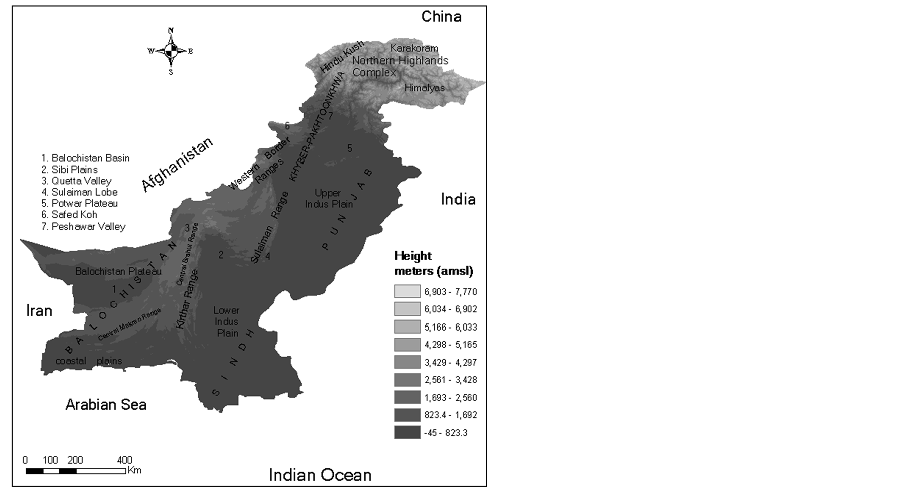
Figure 2. Detail of regions and landforms in Pakistan.
the period of 1950-2000 with grid resolution of 2.5˚ × 2.5˚ at global scale. Figures 3-5 are based on respective simulated results of EOF-1, EOF-2 and EOF-3. EOF1 is the leading eigenvector, which indicates the largest variability of the covariance matrix. The EOF2 is the second eigenvector, and it means the second-largest variability of the raw data’s distribution structure similarly, EOF3, which is the third eigenvector and it means the third largest variability of the covariance matrix [20] . The depicted results in each set of EOF are shown with the help of Pakistan map displays spatial coefficient patterns, a time series, and correlation coefficient at SLP and relationship at 500-hPa height. The correlation coefficient is well defined especially where it exceeds 95% significance level, marked by blue patches on the maps at SLP and 500-hPa levels.
3. Results and Discussion
EOF-1: Figures 3(a)-(e) display the results of leading EOF. Reference to Figure 3(a) the spatial variation is consistent in surface air temperature as a main feature with variance factor of 30.24%. The rugged parts in
 (a)
(a) (b)
(b) (c)
(c)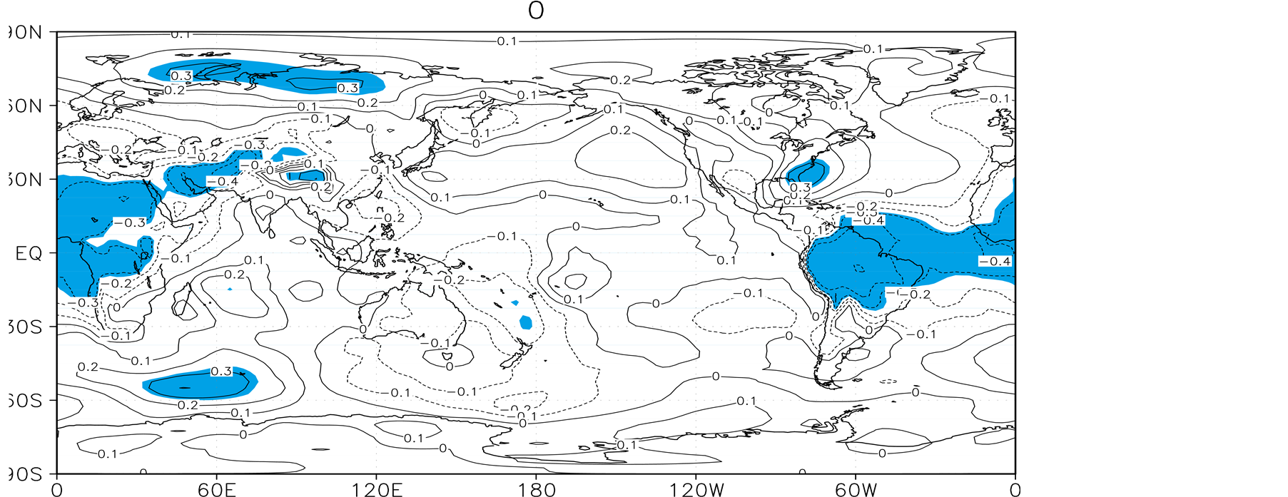 (d)
(d)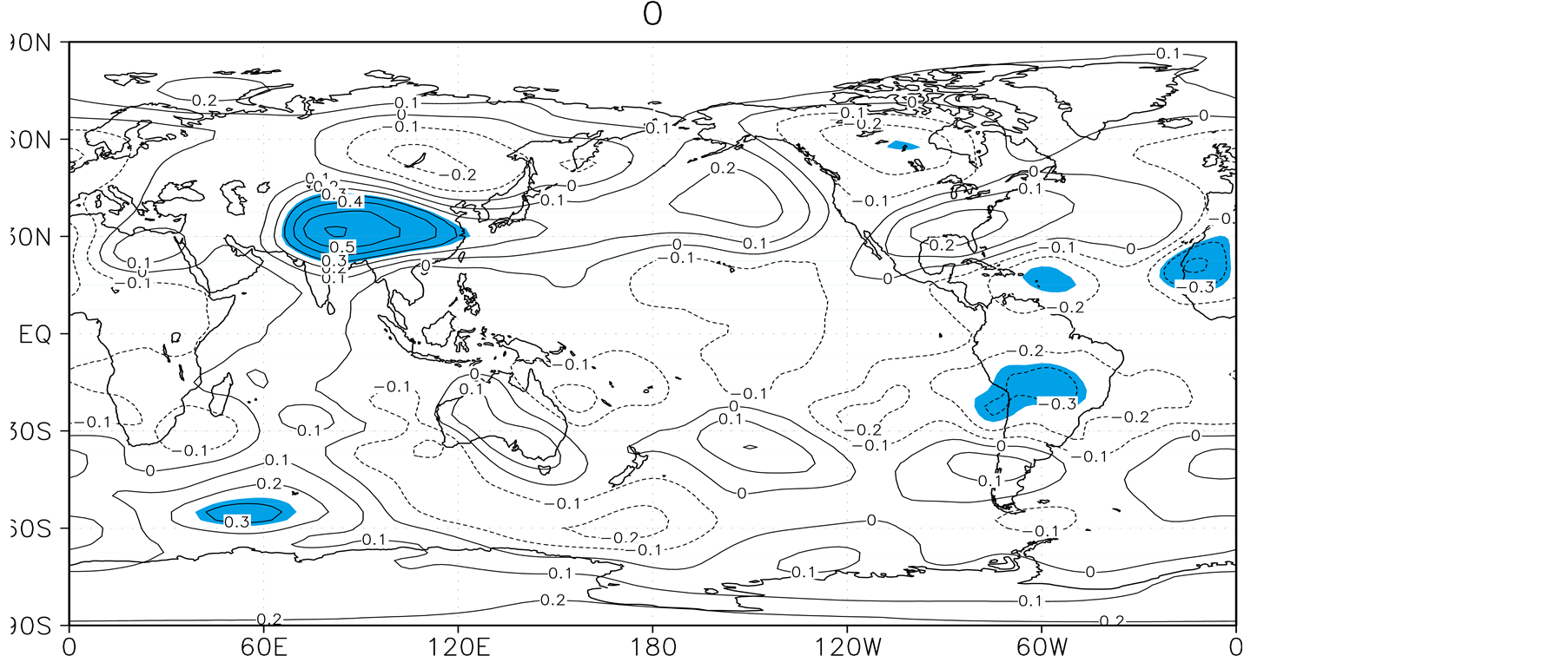 (e)
(e)
Figure 3. (a) Distribution of temperature coefficient shows spatial variations in different areas of Pakistan; (b) Time series of the January surface temperature anomalies in Pakistan (1950- 2000); (c) Comparison between January temporal trend (green lines) and average temperature (black lines) (1950-2000); (d) configures the teleconnections at SLP at global scale in association with January temperatures of the study area over the period of 1950-2000; (e) is the representative of global teleconnection at 500-hPa anomalous field over the period of 1950-2000 in relation to January temperature in Pakistan.
 (a)
(a) (b)
(b)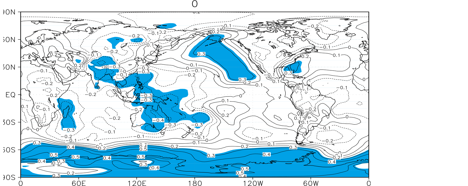 (c)
(c)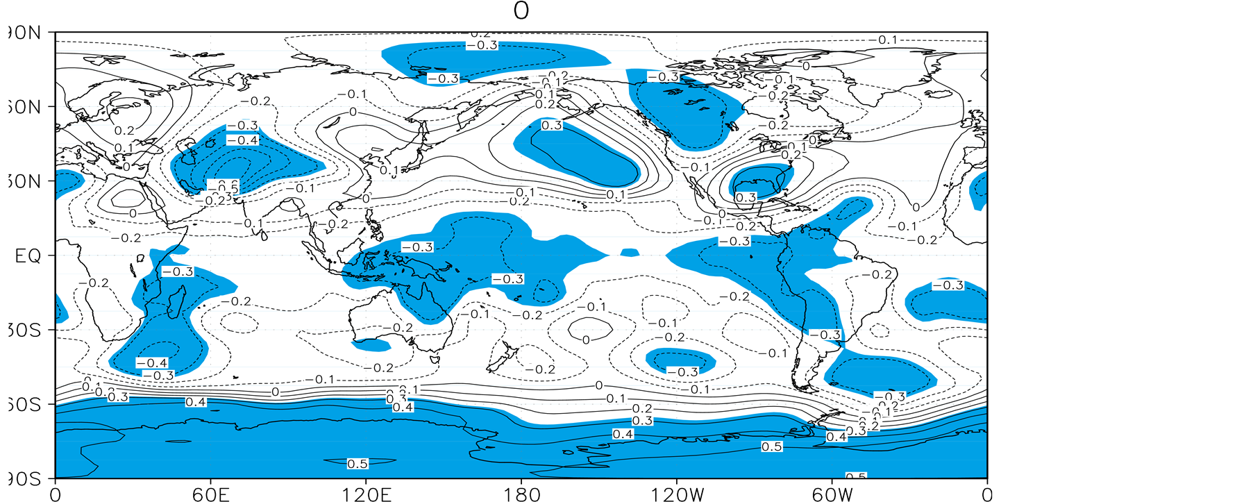 (d)
(d)
Figure 4. (a) Distribution of temperature coefficient shows consistent spatial variations in different territories of Pakistan (January 1950-2000); (b) Time series of the surface temperature anomalies (January 1950-2000); (c) configures the teleconnections at SLP in association with study area temperature; (d) Simulated correlation coefficient over the period of 1950-2000 configures the teleconnections at 500-hPa field.
 (a)
(a) (b)
(b)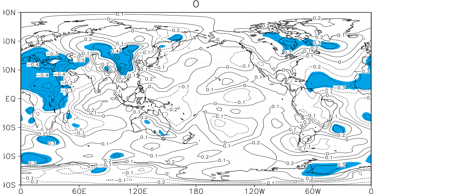 (c)
(c)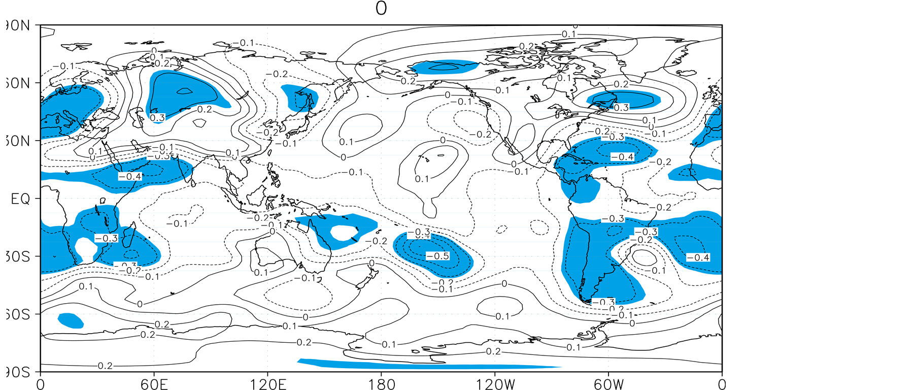 (d)
(d)
Figure 5. (a) Distribution of temperature coefficient shows spatial variations in different territories of Pakistan; (b) Time series of the surface temperature anomalies in Pakistan (January 1950-2000); (c) Correlation coefficient to EOF3 from 1950-2000 in January configures the teleconnections at SLP in association with study area temperature; (d) Simulated correlation coefficient to EOF3 over the period of 1950-2000 configures the teleconnections at 500-hPa field in association with January temperatures in Pakistan.
northern and western parts of the country show significant temperature variability discretely marked over the different areas including coastal built along Arabian Sea, Balochistan Plateau, Sulaiman Ranges Indus Plains, western border ranges. The northern lofty mountains registers steep variations, it means that variability is more obvious in rugged mountainous landscapes. The temporal analysis (Figure 3(b)) shows the characteristics of interannual temperature variability with no strong signal of interdecadal change. However, in 1960s, and 1990s some tacit signatures of interdecadal changes do exist. On the contrary, the interannual signatures were continued throughout the study period. In twenty years, January was warm while January temperatures were below reference point in twenty-three years and the rest of the years were close to normal. The validation through comparison (Figure 3(c)) reflects that interannual variability and average temperature show the r value of about 0.75 and exceeds the 0.01 confidence level.
Based on Figure 3(d) the January temperature has significant relation with SLP, the mode in January shows 95% significance in northern tropical Atlantic and Mediterranean region extending through Middle East to the proximity of the study area. The said areas are mostly under the influence of WDs in winter [21] . Thus, the pressure trough of these localities has influence on the January temperatures of Pakistan. The January temperature in Pakistan has significant relation with atmospheric condition at 500-hpa in South Asia, most of China especially Tibetan Plateau where highest correlation values are observed. The Mediterranean region also configures relationship with study area temperature but not that much strong as it was at SLP. Hence, the trough condition at low level in winter is more active to influence the January surface temperature in Pakistan.
EOF-2: Figures 4(a)-(d) Display the results of EOF2. The spatial variation in temperature from south (north) to north (south) over Pakistan (Figure 4(a)) appears as salient feature with variance factor of about 22.77%. Generally the variation pattern are (−), (+), (−) and then (+). The variation is persistent as one proceeds from southwestern coastal belt to the interior of Balochistan Plateau, which is bordered by Central Makran Range in the south and Central Brahui Range in the east (Figure 2). Positive and negative coefficient pattern prevail over the northeast and northwest corner of the country in lofty mountains. It is worthy to not that this is the most sensitive area in response to climate change and affecting the annual runoff in Indus river basin, the bread basket of Pakistan which supports the agriculture and hydro power generation for about 160 million national population. The northern Pakistan has the world famous and big valley glaciers like Siachin, Batura and Baltora are facing acute depletion, various studies show [22] -[25] that most of the valley glaciers have been subjected to ablation in the extreme north in second half of the Twentieth Century particularly in the last decade. The temporal variably of January temperature show spiky behavior (Figure 3(b)) dominated by interannual variations simultaneously projects an impression of decadal signal of change in the 1950s, 1960s and 1970s. Balochistan comprised of about 41% national territory where January is warmer in 1958, 1960, 1963, 1965, 1966, 1969-1970, 1976, 1979, 1981, 1982-1987, 1989-1995, 1998 and 2000, the same years are also warmer in rest of Pakistan like in KPK, FATA and western parts of Sindh. On the contrary January temperatures are below average in these areas in the years of 1950-1955, 1957, 1959, 1962, 1964, 1967-1968, 1971-1975, 1977-1978, 1984, 1989, 1996-1997 and 1999. In this situation, Indus Plains show less significant relationship with the above said interannual variability.
Reference to correlation coefficient at SLP (Figure 4(c)) the WPB, Bay of Bengal and India shows strong relation with the January temperature variability in Pakistan, simultaneously the persisting situation over the northern tropical Atlantic extending to Mediterranean region, Middle East and Central Asia also remain important but not as strong as in WPB. An isolated patch of significant relation has been located over the Madagascar and surrounding in the Indian Ocean. The most important is the area in the proximity of Pakistan likes Middle East, Central Asia and Tibetan plateau where high confidence level is achieved at 500-hPa level. The westerly waves in the middle latitude of northern hemisphere seem to be important in association with January temperatures in Pakistan. The regressed 500-hPa in the tropical WPB, this is the area where from almost El Niño (La Niña’s) impact originates. Both geopotential levels (SLP & 500 hPa) configure the teleconnection signals that persist over the Antarctic region.
EOF-3: Figures 5(a)-(d) display the results of EOF3 analysis. In this case, the variance associated with the spatial distribution of temperature shows consistent change from negative (region) to positive (region) and again taken over by negative pattern examined from south to north with a variance factor of 14.26% (Figure 3(a)). It is indicative of persistent spatial variability in temperature over the study domain additionally the variation gradient is steeper in the mountainous regions especially in western rugged parts. The temporal anomalies reflect interannual variability but not that much strong as observed in case of EOF1 and EOF2. However, decadal changes have been captured, the decade of 1950 is cool in Balochistan and northern lofty mountains, warmer in Sulaiman ranges and Indus Plains. Except few years 1960s, 1970s, 1980s and 1990s are warmer decades in Balochistan while these decades are cool in Sulaiman ranges and Indus Plains.
The Mediterranean region with south Europe and north Africa extending up to tropical Atlantic basin labeled with high significant values at SLP (Figure 5(c)). The other significant area over the continental eastern Asia is extending up to Siberia that might indicate relation with Siberian high-pressure region. The strong significant areas at 500-hPa are the Arabian Sea with surrounding and areas in the tropical WPB. The signatures with strong correlation over Europe and Siberia might represent the relation with midlatitude westerly flow.
4. Conclusions
Based on EOF analysis the spatial-temporal dynamics of January temperatures over the time of 1950-2000 have been observed with regional details. In study locus, the mountainous regions show more obvious temperature variability than Indus Plaines. The result supports that interannual variability is more pronounced than the interdecadal changes. However, some interdecadal changes have been traced in the last EOF mode.
The teleconnections in the proximity of the study area seem to be instrumental to trace the variability of temperature. In this context, Mediterranean area, Middle East, central Asia and Arabian Sea with its surrounding were more significant. Also the January temperature shows significant relationship with other prominent global teleconnections as appear at SLP and 500 hPa geopotential levels like over northern tropical Atlantic Basin, Warm pool region of the Pacific Basin and Central Asian High. In addition, the WPB is the considerable area that has high correlation with the study domain. The impression of relationships with Antarctic Oscillations (AAO) needs further scientific investigation because this region was captured by almost all three EOF with considerable level of confidence. Conclusively the observed spatial-temporal variability has strong relation with the trough condition in January associated with WDs that prevail over the Mediterranean region and surroundings. The middle latitude westerly flow at 500 hPa field seems to be strong factor which influences the surface temperature in January.
It is clear from the simulated results in all three EOF that the January temperature variability in Pakistan has considerable relation with atmospheric circulation at SLP and 500-hPa at different places in both the terrestrial hemispheres. In this context the tropical Atlantic ocean, northern Indian Ocean including Arabian Sea, western tropical Pacific basin including warm pool region significantly interact with study area. This study could be useful as base line information for further scientific inference in climate change studies addressing Pakistan.
Acknowledgements
Thanks go to PMD by providing the data for this academic research work. I am grateful to Dr Ghulam Rasul Chief Meteorologist PMD, Islamabad for his help and cooperation.
References
- Trenberth, K.E., Jones, P.D., Ambenje, P., Bojariu, R., Easterling, D., Klein T.A., Parker D., Rahimzadeh, F., Renwick, J.A., Rusticucci, M., Soden, B. and Zhai, P. (2007) Observations: Surface and Atmospheric Climate Change. In: Solomon, S., Qin, D., Manning, M., Chen, Z., Marquis, M., Averyt, K.B., Tignor, M. and Miller, H.L., Eds., Climate Change 2007: The Physical Science Basis. Contribution of Working Group I to the Fourth Assessment Report of the Intergovernmental Panel on Climate Change, Cambridge University Press, Cambridge, UK and New York, USA.
- IPCC, Climate Change (2001) The Scientific Basis. Cambridge University Press, Cambridge.
- IPCC (2013) Summary for Policymakers. In: Stocker, T.F., Qin, D., Plattner, G.-K., Tignor, M., Allen, S.K., Boschung, J., Nauels, A., Xia, Y., Bex, V. and Midgley, P.M., Eds., Climate Change: The Physical Science Basis. Contribution of Working Group I to the Fifth Assessment Report of the Intergovernmental Panel on Climate Change, Cambridge University Press, Cambridge, UK and New York, USA.
- Knapp, P.A. and Yin, Z.Y. (1996) Relationships between Geopotential Heights and Temperature in the South-Eastern US during Wintertime Warming and Cooling Periods. International Journal of Climatology, 16, 195-211.
http://dx.doi.org/10.1002/(SICI)1097-0088(199602)16:2<195::AID-JOC1>3.0.CO;2-A - Houghton, J. (2004) Global Warming: The Complete Briefing. Cambridge University Press, Cambridge, 124-140. http://dx.doi.org/10.1017/CBO9781139165044
- Qian, W. and Qin, A. (2006) Spatial-Temporal Characteristics of Temperature Variation in China. Meteorology and Atmospheric Physics, 93, MAP-0/758, 1-16.
- Abdou, A. (2014) Temperature Trend on Makkah, Saudi Arabia. Atmospheric and Climate Sciences, 4, 457-481. http://dx.doi.org/10.4236/acs.2014.43044
- Houghton, J.T., Jenkins, G.J. and Ephraums, J.J. (Eds.) (1990) Climate Change: The IPCC Scientific Assessment. Cambridge University Press, Cambridge, MA.
- Aigang, L.U., Deqian, P., Jianping, G.E., et al. (2006) Effect of Landform on Seasonal Temperature Structures across China in the Past 52 years. Journal of Mountain Science, 3, 158-167.
- Huang, Y. and Qian, Y. (2007) Analysis of the Simulated Climatic Characters of the South Asia High with a Flexible Coupled Ocean-Atmosphere GCM. Advances in atmospheric Sciences, 24, 136-146.
- Thornton, P.E., Running, S.W. and White M.A. (1997) Generating Surfaces of Daily Meteorology Variables over Large Regions of Complex Terrain. Journal of Hydrology, 190, 214-251.
http://dx.doi.org/10.1016/S0022-1694(96)03128-9 - Daly, C., Gibson, W.P., Taylor, G.H., Johnson, G.L. and Pasteris, P. (2002) A Knowledge-Based Approach to the Statistical Mapping of Climate. Climate Research, 22, 99-113.
http://dx.doi.org/10.3354/cr022099 - Braud, I. and Obled, Ch. (1991) On the Use of Empirical Orthogonal Function (EOF) Analysis in the Simulation of Random Fields. Stochastic Hydrology and Hydraulics, 5, 125-134.
http://dx.doi.org/10.1007/BF01543054 - Wallace, J.M. and Gutzler, D.S. (1980) Teleconnections in the Geopotential Height Field during the Northern Hemisphere Winter. Monthly Weather Review, 109, 784-812.
http://dx.doi.org/10.1175/1520-0493(1981)109<0784:TITGHF>2.0.CO;2 - Wang, C.Z., Enfield, D.B., Lee, S.-K. and Landsea, C.W. (2006) Influences of the Atlantic Warm Pool on Western Hemisphere Summer Rainfall and Atlantic Hurricanes. Journal of Climate, 19, 3011-3028. http://dx.doi.org/10.1175/JCLI3770.1
- Levitus, S., Antonov, J.I., Boyer, T.P. and Stephens, C. (2000) Warming of the World Ocean. Science, 287, 2225-2229. http://dx.doi.org/10.1126/science.287.5461.2225
- Wang, C., Xie, S.-P. and Carton, J.A. (2004) A Global Survey of Ocean-Atmosphere and Climate Variability. In: Wang, C., Xie, S.-P. and Carton, J.A., Eds., Earth Climate: The Ocean-Atmosphere Interaction, Geophysical Monograph, 147, AGU, Washington D.C., 1-19.
- Ahmad, I., Sun, Z., Deng, W. and Ambreen, R. (2010) Trend Analysis of January Temperature in Pakistan over the Period of 1961-2006: Geographical Perspective. Pakistan Journal of Meteorology, 7, 11-22.
- Hijmans, R.J., Camerone, S.E., Parra, J.L., Jones, P.G. and Jarvis, A. (2005) Very High Resolution Interpolated Climate Surfaces for Global Land Areas. International Journal of Climatology, 25, 1965-1978. http://dx.doi.org/10.1002/joc.1276
- Jolliffe, I.T. (1986) Principal Component Analysis. Springer Verlag, Berlin, 271 p.
http://dx.doi.org/10.1007/978-1-4757-1904-8 - Syed, F.S., Giorgi, F., Pal, J.S. and King, M.P. (2006) Effect of Remote Forcings on the Winter Precipitation of Central Southwest Asia Part 1: Observations. Theoretical and Applied Climatology, 86, 147-160. http://dx.doi.org/10.1007/s00704-005-0217-1
- Rasul, G., Qin, D. and Chaudhry, Q.Z. (2008) Global Warming and Melting Glaciers along Southern Slopes of HKH Ranges. Pakistan Journal of Meteorology, 5, 63-76.
- Butt, M.J. and Iqbal, M.F. (2009) Impact of Climate Variability on Snow Cover: A Case Study of Northern Pakistan. Pakistan Journal of Meteorology, 5, 53-64.
- Rasul, G. and Chaudhry, Q.Z. (2007) Global Warming and Expected Snowline Shift along Northern Mountains of Pakistan. Proceedings of 1st Asiaclic Symposium, Yokohama, 20-22 April 2006.
- Bashir, F. and Rasul, G. (2010) Estimation of Average Snow Cover over Northern Pakistan. Pakistan Journal of Meteorology, 7, 63-69.
NOTES

*Corresponding author.