Atmospheric and Climate Sciences
Vol. 2 No. 2 (2012) , Article ID: 18820 , 15 pages DOI:10.4236/acs.2012.22017
Trends in Latent and Sensible Heat Fluxes over the Southern Ocean
1Applied Hydrometeorological Research Institute, Nanjing University of Information Science & Technology, Nanjing, China
2Polar Research Institute of China, Shanghai, China
3National Marine Environment Forecast Center, Beijing, China
4Michigan State University, East Lansing, USA
5National Center for Atmospheric Research, Boulder, USA
Email: yulejiang@sina.com.cn
Received December 12, 2011; revised January 16, 2012; accepted February 5, 2012
Keywords: Southern Ocean; Antarctic Oscillation; Pacific-South America Teleconnection; El Niño-Southern Oscillation; Heat Flux
ABSTRACT
In this study, the trends in latent and sensible heat fluxes (LHF and SHF) over the Southern Ocean (oceans south of 35˚S) and the contributions of the Antarctic Oscillation (AAO), the Pacific-South America teleconnection patterns (PSA1 and PSA2) and The El Niño-Southern Oscillation (ENSO) to these heat fluxes were investigated using the Objectively Analyzed Air-Sea Fluxes (OAFlux) dataset from 1979 to 2008. Significant positive annual trends in LHF occur over the Agulhas Current, the Brazil Current, the oceans in the vicinity of New Zealand and southern Australia, and the eastern Pacific Ocean near between 35˚S and 40˚S. Significant negative seasonal trends occur in LHF which differ among the four seasons. The spatial pattern and seasonal variation of the trends in SHF over the Southern Ocean are similar to those of LHF. The spatial patterns of the trends in LHF and SHF caused by the AAO, PSA1, PSA2 and Southern Oscillation Index (SOI) indices show a wave-like feature, varying with different seasons, that can be explained by the anomalous meridional wind associated with the four indices. The above four indices account for a small portion of the trend in LHF and SHF. The residual trends in LHF over the Southern Ocean may be explained by a climate shift in the late 1990s for the four seasons. But the residual trends in SHF over the Southern Ocean are not associated with the climate shift.
1. Introduction
The Southern Ocean (oceans south of 35˚S) plays a critical role in the variability of weather and climate at southern high latitudes through heat and moisture transfer between the upper ocean and atmospheric boundary layer [1,2]. Monitoring heat transfer between the ocean and the atmosphere is thus crucial for understanding the climate system at southern high latitudes. Latent and sensible atmosphere-ocean heat fluxes (LHF and SHF) exhibit larger interannual and spatial variability than other heat fluxes [3,4]. Hence, it is important to investigate longterm LHF and SHF over the Southern Ocean. Here, positive flux is upward, i.e. heat is transferred from ocean to atmosphere.
Previous research has shown that The El Niño-Southern Oscillation (ENSO) and the Antarctic Oscillation (AAO) influence LHF and SHF over the Southern Ocean [5-10]. Positive (negative) AAO is associated with anomalous negative (positive) heat fluxes over the eastern Indian Ocean and the central Pacific Ocean, with anomalous positive (negative) heat fluxes over other regions of the Southern Ocean, which can be explained by meridional wind anomalies associated with the AAO. Verdy et al. (2006) found that LHF and SHF variability induced by ENSO occurs principally over the Pacific Southern Ocean and is related to anomalous meridional wind associated with ENSO [7].
In recent decades, the environmental variables of the Southern Ocean have undergone pronounced changes. Gille (2002) found that mid-depth Southern Ocean temperatures have risen 0.17˚C between the 1950s and the 1980s [11]. Chapman and Walsh (2007) found that from 1958 to 2002 different regions of the Southern Ocean display different trends in surface air temperature [12]. Cavalieri and Parkinson (2008) reported the trends for the Southern Hemisphere as a whole and for five sectors [13]. They found that the trend in total Antarctic Sea Ice extent (SIE) increased slightly from 0.96% ± 0.61% decade–1 for the 20-year period of 1979 to 1998 to 1.0% ± 0.4% decade–1 for the 28-year period of 1979 through 2006, with contrasting changes in the sector trends. Yang et al. (2006) detected a positive trend of Southern Ocean surface wind stress from 1980 through 1999 and its close linkage with spring Antarctic ozone depletion [14]. Thompson and Solomon (2002) presented evidence that recent trends in the Southern Hemispheric circulation can be interpreted as a positive trend in the Southern Hemispheric Annular Mode, with stronger westerly flow over the Southern Ocean [15].
Overall, few papers have been published on trends in LHF and SHF over the Southern Ocean. Moreover whether LHF and SHF over the Southern Ocean have changed, and if so, which meteorological variables and largescale circulation indices influence them need to be explored.
This paper investigates the extent to which AAO, the Pacific-South America teleconnection patterns (PSA1 and PSA2), and ENSO, as well as surface meteorological variables, can account for the recent trends in LHF and SHF over the Southern Ocean. Section 2 describes the data sources and analytical methods. The contributions of these indices to trends in Antarctic sea ice are discussed in Section 3. The effects of input variables on the trends in LHF and SHF are discussed in Section 4. Conclusions and further discussion are given in Section 5.
2. Data and Methods
2.1. Data
The monthly LHF and SHF are derived from the Objectively Analyzed Air-Sea Fluxes (OAFlux) dataset with a spatial resolution of 1.0 degree × 1.0 degree from January 1979 to December 2008 [16]. To obtain the best possible global daily estimates for wind speed at 10 m, and sea surface temperature (SST), air temperature and humidity at 2 m, the OAFlux synthesis uses an objective analysis technique to combine surface meteorological fields from satellite remote sensing and reanalysis outputs produced from the National Centers for Environmental Prediction (NCEP) and the European Centre for Medium Range Weather Forecasts (ECMWF) as well as an advanced objective analysis [17]. The OAFlux project uses the state-of-the-art Coupled Ocean Atmosphere Response Experiment (COARE) bulk flux algorithm version 3.0 to compute the fluxes. Yu et al. (2008) indicate that the OAFLux estimates are unbiased and have a smaller mean error than the NCEP1, NCEP2, and ECMWF flux algorithms [17]. In addition, wind speed at 10 m, air humidity at 2 m, and SST are also obtained from the OAFlux data. To facilitate the comparison during four austral seasons, autumn (March-May), winter (June-August), spring (September-November), and summer (December-February) are defined.
2.2. Methods
The AAO, PSA1 and PSA2 indices are defined as the standardized time coefficients for leading three modes of an empirical orthogonal function (EOF) analysis of monthly sea level pressure poleward of 20˚S (Figure 1). Total linear trends are obtained as the slope of a linear least squares fit at each grid point at specific periods. The trends that are linearly congruent with the monthly AAO, PSA1, PSA2, and SOI indices can be obtained in the following manner [6]:
1) Regressing monthly values of the time series of each grid point onto the AAO index.
2) Multiplying the resulting regression coefficients by the linear trend in the AAO index.
3) Carrying out the same procedure for the PSA1, PSA2, and SOI indices.
For the interannual time scales, PSA1 and PSA2 are associated with the ENSO [18]. We also calculated seasonal correlation coefficients between the SOI index, and the PSA1 and PSA2 indices during the four seasons: 0.52 and 0.42 in autumn, 0.70 and 0.21 in spring, 0.12 and –0.03 in summer and 0.10 and –0.01 in winter, with confidence levels exceeding 95% for PSA1 in autumn and spring, and PSA2 in autumn. The correlation coefficients between the AAO index and the SOI index during the four seasons are less than the 95% confidence level. Therefore, the overlap between the ENSO and the PSA1 is deleted in calculating the residual trend by the relation:
 (1)
(1)
where cov(SOI, PSA1) and var(SOI) are the covariance between the ENSO and PSA1, and the variance of the ENSO, respectively.
By this method, the part of PSA2 (PSA2*) that does not include the ENSO can also be obtained. The residual trend is defined as the trend obtained by subtracting the trends in the AAO, PSA1*, PSA2*, and SOI indices from the total trend.
The trends in the AAO, PSA1, PSA1*, PSA2, PSA2* and SOI indices during the four austral seasons are listed in Table 1. Only the springtime trend in the PSA1 index exceeds the 95% confidence level. Although the trend in AAO is positive from 1979 to 2008, it does not reach the 95% confidence level. Previous studies indicated that AAO has a significant positive trendbecause their AAO indices included time series before 1979 [5,19,20]. We compare different trends in the AAO indices defined by Gong and Wang (1999) between from 1949-1978 and
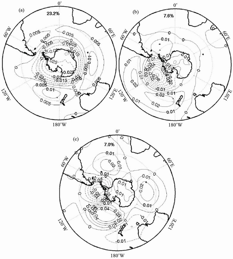
Figure 1. Spatial distributions of the leading three EOF modes of mean sea level pressure (southward of 20˚S): The (a), (b), and (c) indicate the first, second and third modes, respectively. The first three modes explain 23.2%, 7.6%, and 7.0% of the total variance, respectively.

Table 1. 30-yr (1979-2008) linear trends in the AAO, PSA1, PSA1*, PSA2* and PSA2 indices (std·dev·30 yr–1). Trends that exceed the 95% threshold are in bold type.
1979-2005 for four seasons [5]. For the period 1949 to 1978, the linear trends in autumn, winter, spring, and summer are 1.34, 1.16, 1.49, and 1.28 std·dev·30 yr–1, respectively; in contrast, from 1979 to 2005 the trends in autumn, winter, spring, and summer are 1.21, 0.51, 0.26 and 1.19 std·dev·30 yr–1, respectively. We see that the trends before 1979 are larger than those after 1979, especially in austral winter and spring. A similar result can be obtained from the comparison of other AAO indices.
3. Seasonal Contribution of Indices
3.1. Trends in Latent and Sensible Heat Fluxes during the Four Seasons
The trends of LHF and SHF over the Southern Ocean during the four seasons are shown in Figures 2 and 3, respectively. In Figure 2, significantly positive trends in LHF occur over the Agulhas Current, the Brazil Current, the ocean in the vicinity of New Zealand and southern Australia, and the eastern Pacific Ocean near between
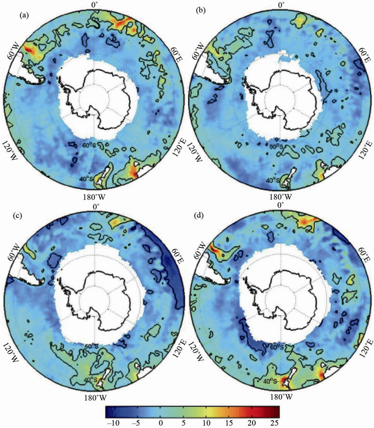
Figure 2. Trends of LHF over the Southern Ocean. (a) Autumn; (b) Summer; (c) Spring; (d) Winter. Units are Wm–2·decade–1. The black lines indicate the regions of >95% confidence level.
35˚S and 40˚S. In contrast, the spatial pattern of the significantly negative trend in LHF differs among the four seasons. In summer, the regions with a negative trend in LHF include the region near the 0˚ longitude line, the southern Indian Ocean, and the ocean to the north of Prydz Bay (68S, 75E). In autumn these are a small part of the southern Atlantic Ocean. In winter the two larger regions are the central southern Indian Ocean and the ocean north of Ross Sea. In spring the largest region lies over the southern Indian Ocean. Additionally, a small section is located over the southwestern Atlantic and eastern Pacific Ocean. The range of the wintertime trend in LHF is the largest in magnitude, from –10 to 25 Wm–2·decade–1, while the smallest magnitude appears in summer from –6 to 16 Wm–2·decade–1. The seasonality of the trend in LHF is in agreement with that of the climatological value of LHF (not shown).
The spatial pattern and seasonal variation of the trend in SHF over the Southern Ocean is similar to those of LHF (Figure 3). But the trend in SHF is smaller with the largest range in winter from –10 to 10 Wm–2·decade–1 and a smaller range in summer from –4 to 5 Wm–2·decade–1. Rouault et al. (2009) also found an increase in LHF and SHF over the Agulhas Current, and related it to an augmentation of SST in this region and the current resulting from an increase in wind stress curl in the South Indian Ocean [21]. The trends in LHF and SHF over the coastal oceans of New Zealand and southern Australia may come from an artifact of satellite observations, because the daily SST used for generating LHF and SHF is partially derived from the Advanced Very High Resolution Radiometer (AVHRR) [22]. In the next section we ex-

Figure 3. Trends of SHF over the Southern Ocean. (a) Autumn; (b) Summer; (c) Spring; (d) Winter. Units are Wm–2·decade–1. The black lines indicate the regions of >95% confidence level.
plore the reason for the trends in LHF and SHF from the point of view of large-scale circulation indices.
3.2. Contributions of Different Indices
The different seasonal trends in AAO, PSA1, PSA2, and SOI can influence their contributions to the trend in LHF and SHF during different seasons. Here we investigate the different effects of the four indices on the trends in LHF and SHF during the same seasons.
Figure 4 shows linear trends in LHF in austral autumn associated with AAO, PSA1, PSA2, and ENSO.
The negative trends related to AAO are distributed over the southwestern and southeastern Pacific Ocean, the central Indian Ocean near 40˚S, and the southern Atlantic Ocean, while elsewhere over the Southern Ocean there is a positive trend. The meridional wind anomalies associated the AAO anomalies lead to surface air temperature anomalies, SST-surface air temperature difference anomalies (Figure 5(a)), and SST-surface air humidity difference anomalies, together with LHF and SHF anomalies (Figures 4(a) and 6(a)). This explanation is supported by the results of Verdy et al. (2006) [7]. A similar analysis was also applied to the PSA1, PSA2, and SOI indices. In Figure 4(b), the negative trends associated with PSA1 are located primarily over the southwestern and southeastern Pacific Ocean, southern Atlantic Ocean, and a small part of the southern Indian Ocean; positive trend regions include the central southern Pacific Ocean, the eastern Atlantic Ocean near 40˚S, the ocean to the south of Australia, and the southern Indian Ocean. The spatial pattern of the PSA2-related trend in LHF exhibits a three-wave structure, which is consistent with
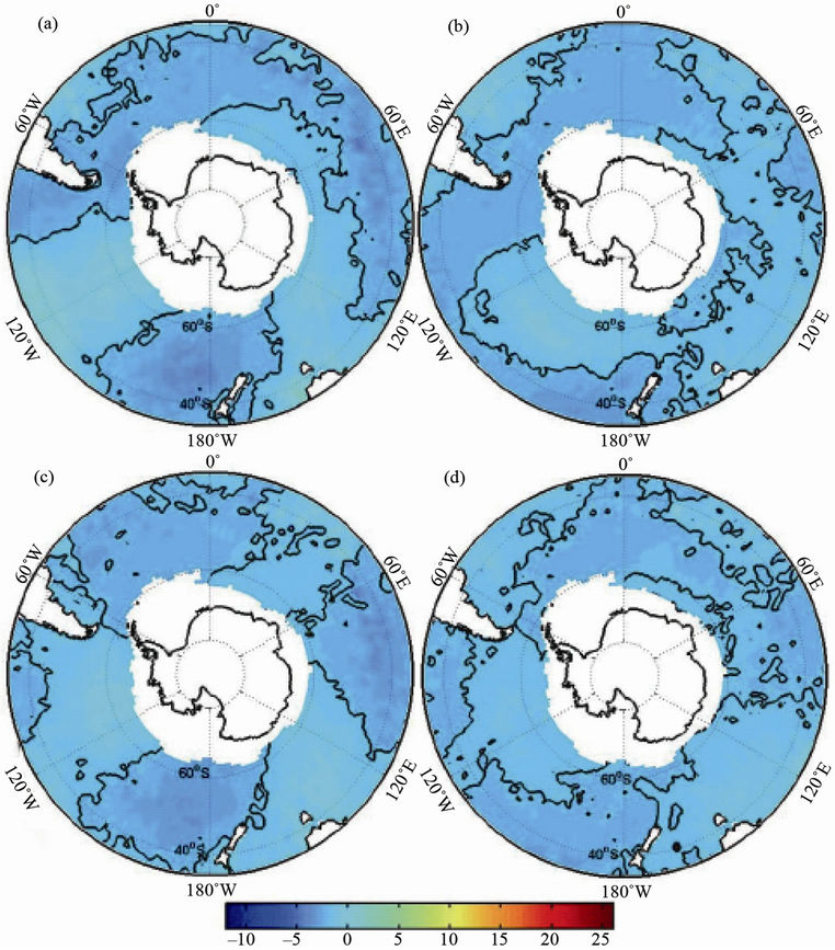
Figure 4. Linear trends in LHF in austral autumn over the period of 1979 through 2008 related to (a) AAO; (b) PSA1; (c) PSA2; (d) SOI. The black solid line indicates the trend of 0. Units are Wm–2·decade–1.
the sea level pressure pattern in Figure 1(c), but a significant trend occurs at the border of positive and negative centers. The spatial pattern of the SOI-related trend in LHF is similar to that of the PSA2-related trend in LHF, but the magnitude of the SOI-related negative trend is less than that of the PSA2-related trend.
The linear trends in SHF in austral autumn have great similarity with those in LHF except for smaller magnitudes. Throughout the year, the four indices vary with different seasons, and their influences on the trend in heat fluxes also vary. Compared with ENSO, the spatial patterns throughout the seasons of the trends in LHF and SHF associated with the other three indices show less variation. We mainly focus on the magnitude of the contributions of the four indices to the trends in LHF and SHF. Tables 2 and 3 display the trend ranges of LHF and SHF caused by the four indices. From Table 2 we can see that the ranges of the trends caused by the four indices differ throughout the year, and have maximum values in different seasons: autumn for AAO; spring for PSA1; autumn for PSA2; winter for SOI. Similar seasonal variation occurs in SHF as shown in Table 3.
In austral autumn, AAO is the major contributor to the
Table 2. Ranges of the trend in LHF associated with the AAO, PSA1, PSA2, and SOI indices. Units are Wm–2·decade–1.
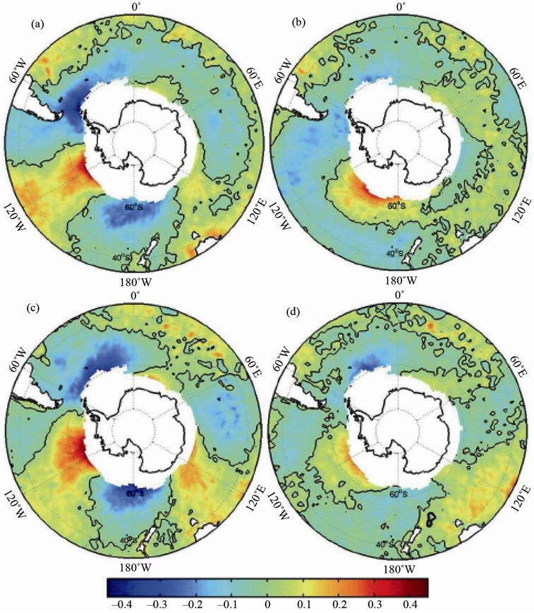
Figure 5. Regression of the difference between SST and air temperature at 2 m anomalies in austral autumn onto (a) AAO; (b) PSA1; (c) PSA2; (d) SOI indices. Units are ˚C. The black solid line indicates the trend of 0.
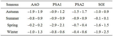
Table 3. Ranges of the trend in SHF associated with the AAO, PSA1, PSA2, and SOI indices. Units are Wm–2·decade–1.
trend in LHF with a range of –2.8 to 3.9 Wm–2·decade–1, but the difference in contribution to the trend in LHF among the other three indices is not large. The smaller difference of the trend in LHF is related to the smaller difference of their indices trends. In austral summer PSA1 exerts the largest influence on the trend in LHF, however the differences between PSA1, and AAO and PSA2 are small. In contrast, the trend in LHF caused by ENSO is only –0.2 to 0.3 Wm–2·decade–1. In spring the contribution of PSA1 to the trend in LHF is more than that of other three indices, with a range of –2.7 to 4.5 Wm–2·decade–1. The magnitude of the trend related to AAO and PSA2 is less than 0.6 Wm–2·decade–1. In winter the impact of ENSO on the trend in LHF greatly exceeds that of the other three indices, with a range of –3.0 to 4.7 Wm–2·decade–1, which is consistent with their indices trends.
The results in Table 3 are similar to those in Table 2, but with smaller values. Additionally we see that in winter the range of the trends in SHF associated with AAO, PSA1, and PSA2 is larger than that in LHF, but this does not occur during the other seasons. The reason may be related to lower humidity in austral winter.
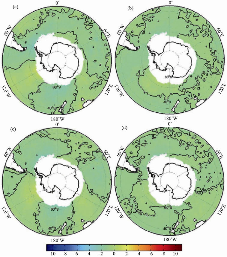
Figure 6. Linear trends in SHF in austral autumn over the period of 1979 through 2008 related to (a) AAO; (b) PSA1; (c) PSA2; (d) SOI. The black solid line indicates the trend of 0. Units are Wm–2·decade–1.
3.3. Residual Trends
We also calculated the residual trend of LHF and SHF during different seasons. The results for LHF are shown in Figure 7. The residual trends of LHF agree with the total trends of LHF except for a small difference in magnitude. This indicates that the four indices explain small trends in LHF over the Southern Ocean, especially over the warm current region, where local effects are more important than large-scale circulations. The magnitude of the residual trends is smaller than that of the total trend with the exception of a negative trend in summer. The decreasing positive trend indicates that LHF over the warm currents is also influenced by the four indices. The largest positive trend explained by the four indices (total trend minus residual trend) of 3.4 Wm–2·decade–1 occurs in summer; the smallest, 0.4 Wm–2·decade–1, occurs in winter. In contrast, the largest negative trend of 2.2 Wm–2·decade–1 appears in spring. Other factors need to be explored to account for the residual trend in LHF.
Figure 8 shows that the spatial patterns of the residual trends in SHF among seasons are similar to those of the residual trends in LHF. Like LHF the residual trends in SHF show little difference with the total trends in SHF. That means the four indices do not explain the trend in SHF and other factors need to be explored. In addition, the maximum and minimum values of total-minus-residual trend in SHF occur in the same seasons as LHF.
4. Effects of Input Variables
To understand the effects of input variables on the trends in LHF and SHF over the Southern Ocean, we examine the trends in the meteorological state variables used as

Figure 7. Residual trends in LHF in (a) Autumn; (b) Summer; (c) Spring; (d) Winter. Units are Wm–2·decade–1. The black solid line indicates the trend of 0.
input in the bulk flux algorithms. Figures 9-11 show the trends in SST, air specific humidity, and wind speed over the Southern Ocean.
Compared with Figures 2 and 3, the trends in SST in Figure 9 are primarily consistent with those in LHF and SHF, especially over the Agulhas and Brazil currents, but a small difference occurs over the mid-latitude Pacific Ocean in autumn and summer. However the trends in specific humidity at 2 m are not in agreement with those in LHF (Figure 10). Over different regions the positive trend in specific humidity corresponds to the positive trend in LHF over the summertime Agulhas current, springtime and wintertime Brazil currents or the negative trend in LHF over the summertime Brazil current, the sea near New Zealand in austral spring, and the springtime and wintertime central Indian Ocean. The trends in wind speed over the Southern Ocean are different among different seasons (Figure 11). In austral autumn and summer, significant increasing trends occur over the Southern Ocean south of 50˚S. In austral spring the Pacific Ocean between 40 and 50˚S displays a remarkable positive trend in wind speed; over the eastern part the LHF and SHF also have increasing trends. In addition, over the region near 0 degrees longitude the wind speed increases. The wintertime trend in wind speed agrees well with that in LHF and SHF; the larger wind speed leads to less stable and larger aerodynamic transfer coefficients [23]. In contrast to air temperature and humidity, the wind speed in austral winter plays a more important role in LHF and SHF.
In summary, among the three variables the largest contributor to the trends in LHF and SHF over the Southern
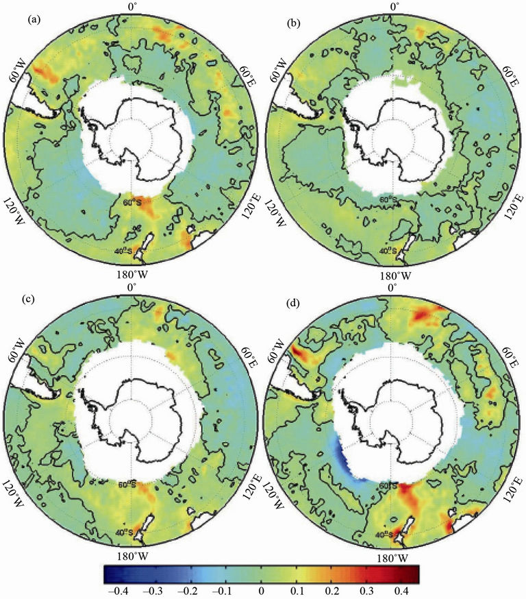
Figure 8. Residual trends in SHF in (a) Autumn; (b) Summer; (c) Spring; (d) Winter. Units are Wm–2·decade–1. The black solid line indicates the trend of 0.
Ocean is SST, while the effect of wind speed is significant only in austral winter. For specific humidity at 2 m, its impact differs for different seasons over different regions.
5. Effects of Recent Global Climate Change
To explore whether recent global climate change influences the residual trends in LHF and SHF, we made EOF analyses of seasonal LHFs and SHFs over the global ocean and the Southern Ocean. Austral autumn and spring coefficients and spatial patterns of the first mode of the LHF over the global oceans and the second mode of LHF over the Southern Ocean are shown in Figure 12. The time coefficients exhibit a shift change in the late 1990s, which also exists in tropical SST, wind and upper atmospheric temperature [24,25]. Before (after) the late 1990s their time coefficients show a negative (positive) anomaly. The correlation coefficients of the climate shift mode explain 12.6% and 15.0% of the variations of LHF over the global oceans in autumn and spring, respectively. In contrast the mode also contributes 12.8% and 12.4% of the variations for LHF over the Southern Ocean in autumn and spring, respectively. Although the first modes of LHF over the Southern Ocean account for more than 16% of the variation, the trends in the time coefficients of the first modes are less significant. The correlation coefficients between time coefficients of the first mode of LHF over the global oceans and the second mode of LHF over the Southern Ocean in autumn and spring are 0.874 and 0.866, respectively. The spatial patterns of the two modes are similar in autumn ((a) and (c)) and in

Figure 9. Trends in SST in (a) Autumn; (b) Summer; (c) Spring; (d) Winter. Units are ˚C·decade–1. The black lines indicate the regions of >95% confidence level.
spring ((b) and (d)). Moreover the spatial patterns of the second mode of LHF over the Southern Ocean in autumn and spring are similar to those of residual trends in autumn and spring. A similar pattern also appears in austral summer (not shown). In austral winter the first mode of LHF over the global oceans and the third mode of LHF over the Southern Ocean are the climate shift modes (Figure 13). The correlation coefficent of time coefficients of the two modes is 0.766. Their spatial patterns are similar to each other and also similar to the residual trend in LHF over the Southern Ocean in winter. Hence the residual trends in LHF over the Southern Ocean may be explained by the climate shift during the 1990s. But for SHFs over the global oceans and the Southern Ocean the climate shift is less significant. The residual trends of SHF over the Southern Ocean need to be explained by other factors.
6. Conclusions
In this study, the contributions of the AAO, PSA1, PSA2 and ENSO to the trends in LHF and SHF over the Southern Ocean were investigated using the OAFlux dataset from 1979 to 2008. Additionally, the effects of SST, air specific humidity, and wind speed on the trends in LHF and SHF are also presented.
Significantly positive trends occur in the spatial patterns of LHF over the Southern Ocean that are consistent among the seasons, while a large difference occurs in the negative trends in LHF. The magnitude of the range of the wintertime trend in LHF is the largest, while the smallest occurs in summer. The spatial pattern and sea-
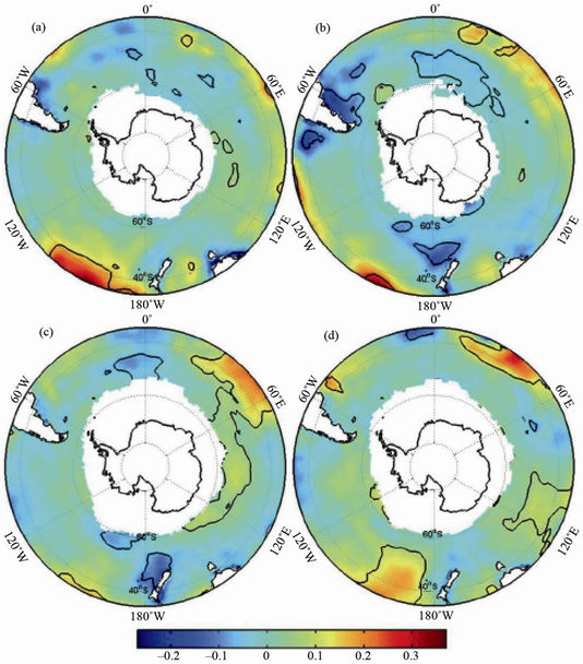
Figure 10. Trends in air specific humidity at 2 m in (a) Autumn; (b) Summer; (c) Spring; (d) Winter. Units are kg–1·decade–1. The black lines indicate the regions of >95% confidence level.
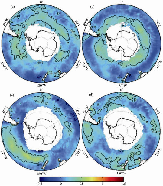
Figure 11. Trends in wind speed at 10m in (a) Autumn; (b) Summer; (c) Spring; (d) Winter. Units are ms–1·decade–1. The black lines indicate the regions of >95% confidence level.

Figure 12. Spatial patterns of the first EOF modes of LHF over the global oceans in autumn (a) and spring (b) and the second EOF modes of LHF over the Southern Ocean in autumn (c) and spring (d); time coefficients of the first EOF modes of LHF over the global oceans (blue line) and the second EOF modes of LHF over the Southern Ocean (red line) in autumn (e); time coefficients of the first EOF modes of LHF over the global oceans (blue line) and the second EOF modes of LHF over the Southern Ocean (red line) in spring (f).
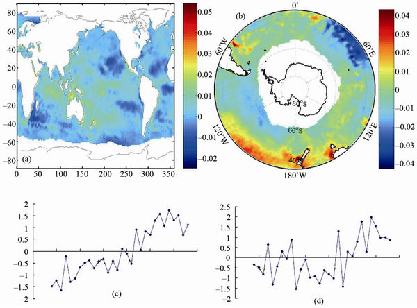
Figure 13. Spatial patterns of the first EOF modes of LHF over the global oceans (a) and the third EOF modes of LHF over the Southern Ocean (b) in winter; time coefficients of the first EOF mode of LHF over the global oceans (c) and the third EOF mode of LHF over the Southern Ocean (d) in winter.
sonal variation of the trend in SHF over the Southern Ocean are similar to those of LHF, but the magnitude is less than that of LHF.
The spatial patterns of the trends in LHF and SHF caused by the AAO, PSA1, PSA2 and SOI indices show a wave-like feature varying with seasons, which can be explained by the anomalous meridional wind associated with the four indices. The seasonality in ENSO is larger than that in the three other indices. The ranges of the trends caused by the four indices differ during the year, and have maximum values in different seasons: for AAO in autumn; for PSA1 in spring; for PSA2 in autumn; for SOI in winter. For the same season, the contributions of the four indices are different from each other. The largest contributors in autumn, summer, spring and winter are AAO, PSA1, PSA1 and ENSO, respectively.
The spatial patterns of residual trends in LHF and SHF are similar to those of the total trends in LHF and SHF. The small difference between total trends and residual trends indicates that the four indices account for only a small portion of the trend in LHF and SHF. Thus we should explore other factors to account for the residual trends in LHF and SHF.
The seasonal variation in the spatial pattern of the SST trend over most of the Southern Ocean is consistent with the trends in LHF and SHF. For wind speed, this is the case only in austral winter. The relationship between specific humidity and LHF is complex and changes with different seasons over different regions. This conclusion needs to be validated with other datasets.
By EOF analyses of LHFs over the global oceans and the Southern Ocean and comparison of the spatial patterns of climate shift modes with the residual trends in LHF over the Southern Ocean, we find that the residual trends in LHF over the Southern Ocean may be explained by the climate shift for four seasons. But this is not the case for SHF.
The significant trends in LHF and SHF may influence the variation in sea ice related to the formation of water mass in the Southern Ocean. Therefore, it would be desirable to explore the climate effect of the trends in LHF and SHF over the Southern Ocean.
7. Acknowledgements
This study was supported by the National Natural Science Foundation (41175010, 40930848 and 41106164), Marine Public Welfare Project (201205007) and National Program on Key Basic Research Project of China (2010CB950301). The National Center for Atmospheric Research is sponsored by the National Science Foundation.
REFERENCES
- J. C. King and J. Turner, “Antarctic Meteorology and Climatology,” Cambridge University Press, Cambridge, 1997. doi:10.1017/CBO9780511524967
- D. Iudicone, S. Speich, G. Madec and B. Blanke, “The Global Conveyor Belt from a Southern Ocean Perspective,” Journal of Physical Oceanography, Vol. 38, No. 7, 2008, pp. 1377-1400. doi:10.1175/2008JPO3519.1
- S. A. Josey, E. C. Kent and P. K. Taylor, “New Insights into the Ocean Heat Budget Closure from Analysis of the SOC Air-Sea Flux Climatology,” Journal of Climate, Vol. 12, No. 9, 1999, pp. 2856-2880. doi:10.1175/1520-0442(1999)012<2856:NIITOH>2.0.CO;2
- S.-H. Chou, E. Nelkin, J. Ardizzone and R. M. Atlas, “A Comparison of Latent Heat Fluxes over Global Oceans for Four Flux Products,” Journal of Climate, Vol. 17, No. 20, 2004, pp. 3974-3989. doi:10.1175/1520-0442(2004)017<3973:ACOLHF>2.0.CO;2
- D. Gong and S. Wang, “Definition of Antarctic Oscillation Index,” Geophysical Research Letters, Vol. 26, No. 4, 1999, pp. 459-462. doi:10.1029/1999GL900003
- D. Thompson and J. Wallace, “Annular Modes in the Extratropical Circulation. Part I: Month-Month Variability,” Journal of Climate, Vol. 13, No. 5, 2000, pp. 1000-1016. doi:10.1175/1520-0442(2000)013<1000:AMITEC>2.0.CO;2
- A. Verdy, J. Marashall and A. Czaja, “Sea Surface Temperature Variability along the Path of the Antarctic Circumpolar Current,” Journal of Physical Oceanography, Vol. 36, No. 7, 2006, pp. 1317-1331. doi:10.1175/JPO2913.1
- A. Verdy, S. Dutkiewicz, M. Follows, J. Marshall and A. Czaja, “Carbon Dioxide and Oxygen Fluxes in the Southern Ocean: Mechanisms of Interannual Variability,” Global Biogeochemistry Cycles, Vol. 21, 2007, 10 p. doi:10.1029/2006GB002916
- F. Vivier, D. Iudicone, F. Busdraghi and Y.-H. Park, “Dynamics of Sea Surface Temperature Anomalies in the Southern Ocean Diagnosed from a 2-D Mixed-Layer Model,” Climate Dynamics, Vol. 34, No. 2, 2009, pp. 153-184. doi:10.1007/s00382-009-0724-3
- J. B. Sallée, K. G. Speer and S. R. Rintoul, “Zonally Asymmetric Response of the Southern Ocean Mixed-Layer Depth to the Southern Annular Mode,” Nature Geoscience, Vol. 3, 2010, pp. 273-279. doi:10.1038/ngeo812
- S. T. Gille, “Warming of the Southern Ocean since the 1950s,” Science, Vol. 295, No. 5558, 2002, pp. 1275-1277. doi:10.1126/science.1065863
- W. L. Chapman and J. E. Walsh, “A Synthesis of Antarctic Temperatures,” Journal of Climate, Vol. 20, No. 16, 2007, pp. 4096-4117. doi:10.1175/JCLI4236.1
- D. J. Cavalieri and C. L. Parkinson, “Antarctic Sea Ice Variability and Trends, 1979-2006,” Journal of Geophysical Research, Vol. 113, 2008, 19 p. doi:10.1029/2007JC004564
- X.-Y. Yang, R. X. Huang and D. X. Wang, “Decadal Changes of Wind Stress over the Southern Ocean Associated with Antarctic Ozone Depletion,” Journal of Climate, Vol. 20, No. 14, 2007, pp. 3395-3410. doi:10.1175/JCLI4195.1
- D. W. Thompson and J. M. Wallace, “Annular Modes in Extratropical Circulation. Part II: Trends,” Journal of Climate, Vol. 13, No. 5, 2000, pp. 1018-1036. doi:10.1175/1520-0442(2000)013<1018:AMITEC>2.0.CO;2
- L. Yu and R. A. Weller, “Objectively Analyzed Air-Sea Heat Fluxes for the Global Ice-Free Oceans (1981-2005),” Bulletin of the American Meteorological Society, Vol. 88, No. 4, 2007, pp. 527-539. doi:10.1175/BAMS-88-4-527
- L. Yu, X. Jin and R. A. Weller, “Multidecade Global Flux Datasets from the Objectively Analyzed Air-Sea Fluxes Project: Latent and Sensible Heat Fluxes, Ocean Evaporation, and Related Surface Meteorological Variables. Woods Hole Oceanographic Institution,” OAFlux Project Technical Report OA-2008-01, Woods Hole, 2008, p. 64.
- K. C. Mo, “Relationships between Low-Frequency Variability in the Southern Hemisphere and Sea Surface Temperature Anomalies,” Journal of Climate, Vol. 13, No. 20, 2000, pp. 3599-3606. doi:10.1175/1520-0442(2000)013<3599:RBLFVI>2.0.CO;2
- D. W. J. Thompson and S. Solomon, “Interpretation of Recent Southern Hemisphere Climate Change,” Science, Vol. 296, No. 5569, 2002, pp. 895-899. doi:10.1126/science.1069270
- G. J. Marshall, “Trends in the Southern Annular Mode from Observations and Re-Analyses,” Journal of Climate, Vol. 16, No. 24, 2003, pp. 4134-4143. doi:10.1175/1520-0442(2003)016<4134:TITSAM>2.0.CO;2
- M. Rouault, P. Penven and B. Pohl, “Warming in the Agulhas Current System since the 1980’s,” Geophysical Research Letters, Vol. 36, 2009, 5 p. doi:10.1029/2009GL037987
- L. Yu, X. Jin and R. A. Weller, “Role of Net Surface Heat Flux in Seasonal Variations of Sea Surface Temperature in the Tropical Atlantic Ocean,” Journal of Climate, Vol. 19, No. 23, 2006, pp. 6153-6169. doi:10.1175/JCLI3970.1
- J. A. Curry and P. J. Webster, Ocean Surface Exchanges of Heat and Fresh Water. “Thermodynamics of Atmospheres and Oceans,” Academic Press, New York, 1999.
- D. E. Harrison and A. M. Chiodi, “Preand Post-1997/1998 Westerly Wind Events and Equatorial Pacific Cold Tongue Warming,” Journal of Climate, Vol. 22, No. 3, 2009, pp. 568-581. doi:10.1175/2008JCLI2270.1
- K.-S. Yun, K.-J. Ha, B. Wang and R. Ding, “Decadal Cooling in the Indian Summer Monsoon after 1997/1998 El Niño and Its Impact on the East Asian Summer Monsoon,” Geophysical Research Letters, Vol. 37, 2010, 6 p. doi:10.1029/2009GL041539