International Journal of Astronomy and Astrophysics
Vol.08 No.02(2018), Article ID:85276,13 pages
10.4236/ijaa.2018.82013
The Geomagnetic Effects of Solar Activity as Measured at Ouagadougou Station
Aristide Marie Frédéric Gyébré, Doua Allain Gnabahou, Frédéric Ouattara
Laboratoire de Recherche en Energétique et Météorologie de l’Espace (LAREME), Université Norbert Zongo (anciennement Université de Koudougou), Koudougou, Burkina Faso
Copyright © 2018 by authors and Scientific Research Publishing Inc.
This work is licensed under the Creative Commons Attribution International License (CC BY 4.0).
http://creativecommons.org/licenses/by/4.0/


Received: March 9, 2018; Accepted: June 11, 2018; Published: June 14, 2018
ABSTRACT
The coronal mass ejections (CMEs) produce by Sun poloidal magnetic fields contribute to geomagnetic storms. The geomagnetic storm effects produced by one-day-shock, two-days-shock and three-days-shock activities on Ouagadougou station F2 layer critical frequency time variation are analyzed. It is found that during the solar minimum and the increasing phases, the shock activity produces both positive and negative storms. The positive storm is observed during daytime. At the solar maximum and the decreasing phases only the positive storm is produced. At the solar minimum there is no three-days-shock activity. During the solar increasing phase the highest amplitude of the storm effect is due to the one-day-shock activity and the lowest is produced by the two-days-shock activity. At the solar maximum phase the ionosphere electric current system is not affected by the shock activity. Nevertheless, the highest amplitude of the storm effect is caused by the two-days-shock activity and the lowest by the one-day-shock activity. During the solar decreasing phase, the highest amplitude provoked by the storm is due to the three-days-shock activity and the lowest by the one-day-shock activity.
Keywords:
CMEs Activity, Shock Activity, F2 Layer Critical Frequency, Geomagnetic Activity, Ionosphere Time Variation

1. Introduction
The Sun has magnetic field that interacts with interplanetary medium by means of its components. The first, namely poloidal magnetic field, is closed and is responsible for coronal mass ejections (CMEs). The second, an opened magnetic field is the source of solar winds (slow solar wind, high stream solar wind, recurrent solar wind and fluctuating solar wind [1] [2] [3] [4] . These solar events provoke four different geomagnetic situations. In fact, 1) the quiet solar wind induces quiet geomagnetic events; 2) the fluctuating wind is responsible for fluctuating geomagnetic activity; 3) the recurrent solar wind causes recurrent geomagnetic activity and 4) CMEs produce shock activity.
As the ionospheric storms are closely associated with the geomagnetic storms [5] [6] , we investigate the geomagnetic storm effect on the ionosphere F2 region. Here, are interest the storms due to CMEs actions. Studies of the other disturbed activities (the recurrent and the fluctuating activities) impacts on the ionosphere F2 region specifically in the African equatorial ionization anomaly (EIA) sector are out of the topic of the present study.
To investigate CMEs action on the ionosphere, Ouagadougou ionosonde station (Lat: 12.4˚N; Long: 358.5˚E; dip: 1.43˚) F2 layer critical frequency (foF2) will be used. Keeping in mind that the response of the ionosphere to storms is rather complicated [5] and comprehensive understanding of nonlinear interaction among the thermosphere, ionosphere and magnetosphere during geomagnetic storms remains a challenge to be identified/to be understood [7] . To contribute to this challenge, the present work investigates the effect on the ionosphere due to CMEs storm activity.
For better investigating the CMEs storm activity on ionosphere, we consider the duration time skill of the storm action on the ionosphere. The storm action duration time skill gives an opportunity to classify the CMEs storms by means of pixel diagrams (see Figure 1). Pixel diagrams show per year an overview of the whole solar geoeffectiveness activity (each type of the solar wind activity [slow, recurrent and fluctuating winds activity] and that of CMEs [8] ).
Our goal through this study is to analyze each type of the shock impacts on

Figure 1. Year 1990 pixel diagram for highlighting each type of activity days.
Ouagadougou station foF2 time variation as recommended by [9] . For doing that, we analyze the pixel diagrams. The analysis of the pixel diagrams let us see the three type of CMEs storm activity called after shock activity as defined by [1] . The starting day of the shock activity on the ionosphere in the pixel diagrams is identified by the date of SSC (Sudden Storm Commencement) indicated by the circle that encircles the geomagnetic index Aa daily values (we give in the Section 2 the detail on that). The retained shocks are: one-day-shock (its action time duration on the ionosphere does not exceed one day), two-days-shock (its action time duration on the ionosphere is more than one day and does not exceed two days) and three-days-shock (its action time duration on the ionosphere is more than two days and does not exceed three days). This point is the novelty of the paper for its storm steady approach differs from those of several papers which treat a particularly shock event (short time variation, effect of storm time different phases with respect to Dst [disturbance storm time] time variation) or address statistical ionosphere F2 layer parameters variability under individual storm activity (e.g. [10] - [32] ). Our objective is, in short term, to present the signature of the storm effect on the equatorial ionospheric currents (equatorial electrojet and equatorial counter electrojet) variability and their strength and in mean and long term to contribute to improve the existing models’ predictability and also to address the space weather issues.
2. Materials and Methods
2.1. The Criteria for Determining the Solar Cycle Phases
For the solar cycle phases determination, we use the following criteria [33] [34] [35] [36] : 1) minimum phase: Rz < 20; 2) ascending phase : 20 ≤ Rz ≤ 100 and Rz greater than the previous year’s value; 3) maximum phase : Rz > 100 [for small solar cycles (solar cycles with sunspot number maximum (Rz max) less than 100) the maximum phase is obtained by considering Rz > 0.8*Rz max]; and 4) descending phase: 100 ≥ Rz ≥ 20 and Rz less than the previous year’s value. In these previous inequations, Rz is the yearly average Zürich sunspot number.
2.2. The Method for Determining the Shock Activity
The geomagnetic storm is defined as a phenomenology of a middle- and low-latitude-geomagnetic variations that can be identified by the intensification of the ring current which is the source of the low-frequency component of storm magnetic variation and quantified by the Dst (disturbance storm time) index [37] . For studying the geomagnetic storm, in this paper, Aa index [38] [39] daily values, are used through pixel diagrams. A pixel diagram helps to select geomagnetic data as a function of the solar activity as described by solar rotation (27 days) [9] . The pixel diagrams consist of 1) plotting the Aa daily values in Bartels diagrams, 2) exhibiting the shock activity (very active spot on solar disc) [1] by showing SSC (sudden storm commencement) dates in these diagrams (indicated by the circle: see Figure 1) because SSC date corresponds to the starting time of geomagnetic storm [6] and 3) adopting a color codes that help to define a geomagnetic activity intensity. According to [1] shock activity is estimated by taking account 2 or 3 disturbed days after SSC date without a recurrence of 27 days during 2, 3 or 4 rotations. By keeping in mind the above conditions for shock activity determination, the analysis of a pixel diagram shows the well-known four geomagnetic classes of activity (quiet, recurrent, fluctuating somewhere name unclear activities and shock activities [three types of shock activity corresponding to (a) one-day-shock (shown by only a day when occurs SSC), (b) two-days-shock ( pointed out by the SSC day with a day after this day) and (c) three-days-shock (identified by the SSC day with two days after this day)]. As noted in introduction section, we only focus our attention on shock activity effects. The other disturbed activities (recurrent activity and fluctuating activities) actions on ionosphere variability are out the topic of the present paper.
In this paper, Ouagadougou station foF2 (three solar cycles (1966-1998) data) values are carried out for each type of shock. For the period involves (1966-1998), we have 323 shock days with 168 days of the one-day-shock, 105 days of the two-days-shock and 50 days of the three-days-shock.
2.3. The Method for Analyzing the Data
Each type of shock values (arithmetic hourly mean values) are plotted in a same panel which corresponds to each solar cycle phase. In order to appreciate the effect of each type of shock, their graphs are compared with that of the quietest time (determined by considering the five quietest days in a month). The error bars shown in the quietest time graph, help us. The error bars applied are carried
out by means of where the variance V is defined by
with mean value and N the total number of observations for a particular dataset.
Before the comparison, with respect to our objectives, foF2 time profiles of each shock are described by reference to [40] profiles (see Figure 2). Figure 2 shows the five typical foF2 time profiles in African EIA (Equatorial Ionization Anomaly) sector. These profiles are called the noon bite out profile or “B” profile (panel a), the morning peak profile or “M” profile (panel b), the dome profile or “D” profile (panel c), the plateau profile or “P” profile (panel d) and the reverse profile or “R” profile (panel e). These profiles can be recorded to the equatorial ionosphere electric currents (equatorial electrojet and equatorial counter electrojet) strength, presence or absence, by reference to the electric current day-to-day time variation under the quiet time condition [41] [42] .
3. Results and Discussion
Figures 3-6 present the statistical arithmetic mean foF2 values diurnal variation under different solar cycle phases for the quietest period (solid curve) and for the three types of shock (one-day-shock (dotted curve), two-days-shock (broken

Figure 2. foF2 profile types after [40] . Panel a concerns noon bite out profile that expresses the signature of strong electrojet; panel b called morning peak profile and exhibits the signature of mean electrojet; panel c profile is dome profile and that of panel d is plateau profile. These two profiles characterized the absence of electrojet. Panel e profile is reverse profile and expresses the signature of strong counter electrojet.

Figure 3. foF2 diurnal variation during sunspot minimum phase under one-day-shock (dotted), two-days-shock (broken), three-days-shock (broken and dotted) and quietest-days (solid).
curve) and three-days-shock (broken and dotted graph). Figure 3 concerns the solar minimum phase, Figure 4 addresses the solar maximum phase, Figure 5 is
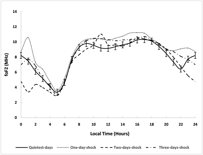
Figure 4. The same as Figure 3 but for solar ascending phase.

Figure 5. The same as Figure 3 but for solar maximum phase.
devoted to the solar increasing phase and Figure 6 concerns the solar decreasing phase.
Figure 3 shows that there is no three-days-shock. One-day-shock profile is the plateau profile with an evening peak at 1800 LT. Two-days-shock curve shows the noon bite out profile with a night time peak at 2000 LT.
The quietest curve highlights the reverse profile. According to foF2 profiles (Figure 2) during the minimum phase, the shock action modifies the ionosphere

Figure 6. The same as Figure 3 but for solar declining phase.
variability shown by the modified foF2 profiles during the storm time with respect to the quietest profile. At low altitude, as the storm maybe due to one or the combined action of thermospherics composition changes, the eastward prompt penetration electric fields, and the equatorward neutral wind [43] - [53] , the storm action can induce change in the ionosphere electric current system. This change produces an effect on ground base magnetic field instruments. According to [41] [42] , the analysis of the signature of the ionosphere electric current found that each foF2 profile can be expressed in term of: 1) the presence or the absence of ionosphere electric current and 2) the strength of ionosphere electric current. In low latitude, the ionospheric electric currents are the equatorial electrojet and the equatorial counter electrojet. Analyzing the Figure 2, according to [40] , from top to bottom we have a strong electrojet, a mean electrojet, an absence of electrojet, an absence of electrojet and a strong counter electrojet, respectively. These results show that to correctly model the shock activity on the ionosphere, during the solar minimum phase, it will be better to take into account each type of shock.
In Figure 3, from daytime to nighttime, the shock activity increases foF2 values. For two-days-shock, we always have except between 0600 LT and 0700 LT where it is the reverse. For one-day-shock we have from 1000 LT to 2300 LT except from 0500 LT to 1000 LT where it is the reverse. It can be concluded that the shock activity usually produces positive storm (a storm foF2 values are superior to those of the quietest periods) [54] which, in this latitude, traduces F2-layers uplifting that is caused by ExB drift-induced [55] . The different observed profiles underline the necessity to treat each type of shock as a specific case for well understand the all mechanism for electrodynamics point of view.
Figure 4 concerns the solar increasing phase. In this figure, 1) the quietest-days profile is a “B” profile with a night time peak at 2400 LT, 2) the one-day-shock profile corresponds to a “R” profile with a night time peak at 2300 LT, 3) a fairly “M” profile for the three-days-shock profile and 4) a “B” profile when is concerned the two-days-shock profile with the predominance morning peak. For the two-days-shock and the three-days-shock profiles, there is no nigh time peak. The analysis of Figure 4 shows a positive storm from 1000 LT to 1900 LT for the one-day-shock, from 1000 LT to 1600 LT for the three-days-shock and between 1100 LT-1300 LT for that concerned the two-days-shock. Negative storm (a storm foF2 values are inferior to those of the quietest periods) appears between 0000 LT and 0500 LT and from 2200 LT to 0000 LT during one-day-shock activity. This is also true for the three-days-shock from 2300 LT to 2400 LT. Reference [53] pointed out that at the low-latitude regions, the nightside ionospheric negative phase is the dominant response to the geomagnetic storm. Here, we found that only the two-days-shock and the three-days-shock activities confirm what have been observed by [53] . This result underlines the necessity to take into account storm time duration in term of day for statistical CMEs storms activity studies.
In general, the critical frequency values can be classified as: .
At daytime as a “B” profile expresses the signature of ExB [56] [57] [58] , the above observations show that only the three-days-shock does not affect this signature. At night time, because a night time peak is due to the signature of the reversal electric field in this latitude [56] [57] [58] [59] we can assert from the profile observation that only the one-day-shock action does not disturbe the effect of the reversal electric.
Figure 5 presents foF2 profiles for the solar maximum phase. It is shown that all foF2 profiles are a “M” profile. This observation points out that the shock activity does not modify the foF2 profile. Consequently, the current system is not affected by the shock action during the solar maximum phase. But at nighttime, even though a nighttime peak is observed in all graphs, the time of its appearance is different: 1900 LT for the one-day-shock, 2300 LT for the three-days-shock and the quietest time and after 2300 LT for the two-days-shock. As a nighttime peak in the foF2 diurnal variation graph is the signature of the reversal electric field in the equatorial region [56] [57] [58] [59] , it can be retained that during the solar maximum phase, the reversal electric field occurs early for the one-day-shock activity and later for the two-days-shock activity periods and remains as during the quietest period for the two-days-shock activity. In general, a positive storm is produced by all shocks except between 2100 LT and 2300 LT during the one-day-shock and the two-days-shock activities. It can be retained from 1000 LT to 1300 LT , from 0200 LT to 1000 LT , from 2100 LT to 2400 LT and between 0000 LT -0200 LT .
Figure 6 concerns the foF2 profiles for the solar decreasing phase. In this figure, the quietest-days profile is a fairly “B” profile with a night time peak at 2200 LT, the one-day-shock profile corresponds to a “R” profile with a night time peak at 2200 LT, a “D” profile with a night time peak at 2300 LT is observed when occurs the two-days-shock and a “B” profile with a fairly night-time peak at 2300 LT is seen when acts the three-days-shock. Figure 6 analysis shows that there is no negative storm. The signature of the reversal electric field is seen one hour after due to the effect of the two-days-shock or the three-days-shock. The one-day-shock activity does not induce this time delay with respect to the quietest period. During daytime, only the two-days-shock activity does not disturb the effect of the signature of ExB.
During daytime, Figure 6 shows that from 0800 LT to 1500 LT . From 1500 to 1700 LT and between 1700 to 1800 LT we have and ,
4. Conclusion
The shock activity due to CMEs is analyzed by taking into account shock time duration, one, two or three days through solar cycle phases. During the period involved, during the solar minimum and the increasing phases shock activity produces positive and negative storms and especially positive storm at daytime. During the two last solar cycle phases only positive storm is produced by the shock activity. Generally, each type of shock modifies ionospheric the electric current system except during the solar maximum phase. The storm effect amplitude expresses the solar cycle dependence and also the shock time duration in day. At daytime, we have 1) for the solar increasing phase ; 2) the during solar maximum phase and for the solar descending phase . Only during the solar minimum there is no three-days-shock activity. These observations point out the necessity to separate the shock activity into the three types of shock activity in term of time duration in day for well-model ionosphere response to shock activity and for space weather study issues.
Cite this paper
Gyébré, A.M.F., Gnabahou, D.A. and Ouattara, F. (2018) The Geomagnetic Effects of Solar Activity as Measured at Ouagadougou Station. International Journal of Astronomy and Astrophysics, 8, 178-190. https://doi.org/10.4236/ijaa.2018.82013
References
- 1. Legrand, J.P. and Simon, P.A. (1989) Solar Cycle and Geomagnetic Activity: A Review for Geophysicists. Part I. The Contributions to Geomagnetic Activity of Shock Waves and of the Solar Wind. Annals of Geophysics, 7, 565-578.
- 2. Simon, P.A. and Legrand, J.P. (1989) Solar Cycle and Geomagnetic Activity: A Review for Geophysicists. Part II. The Solar Sources of Geomagnetic Activity and Their Links with Sunspot Cycle Activity. Annals of Geophysics, 7, 579-594.
- 3. Richardson, I.G., Cliver, E.W. and Cane, H.V. (2000) Sources of Geomagnetic Activity over the Solar Cycle: Relative Importance of Coronal Mass Ejections, High-Speed Streams, and Slow Solar Wind. Journal of Geophysical Research, 105, 18200-18213. https://doi.org/10.1029/1999JA000400
- 4. Richardson, I.G. and Cane, H.V. (2002) Sources of Geomagnetic Activity during Nearly Three Solar Cycles (1972-2000). Journal of Geophysical Research, 107, 1187. https://doi.org/10.1029/2001JA000504
- 5. Sahai, Y., Shiokawa, K., Otsuka, Y., Ihara, C., Ogawa, T., Igarashi, K., Miyazaki, S. and Saito, A. (2001) Imaging Observations of Midlatitude Ionospheric Disturbances during the Geomagnetic Storm of February 12, 2000. Journal of Geophysical Research, 106, 24481-24492. https://doi.org/10.1029/2000JA900169
- 6. Matsushita, S. (1959) A Study of the Morphology of Ionospheric Storm. Journal of Geophysical Research, 64, 305-320. https://doi.org/10.1029/JZ064i003p00305
- 7. Mendillo, M. (2006) Storms in the Ionosphere: Patterns and Processes for Total Electron Content. Reviews of Geophysics, 44, RG4001. https://doi.org/10.1029/2005RG000193
- 8. Ouattara, F. and Amory Mazaudier, C. (2009) Solar-Geomagnetic Activity and Aa Indices toward a Standard Classification. Journal of Atmospheric and Solar-Terrestrial Physics, 71, 1736-1748. https://doi.org/10.1016/j.jastp.2008.05.001
- 9. Gyébré, A.M.F., Ouattara, F., Kaboré, S. and Zerbo, J.L. (2015) Time Variation of Shock Activity Due to Moderate and Severe CMEs from 1966 to 1998. British Journal of Science, 13, 1-7.
- 10. Obayashi, T. (1964) Morphology of Storms in the Ionosphere. In: Odishaw, H., Ed., Geophysical Research 1, MIT Press, Cambridge, 335-366. https://doi.org/10.5636/jgg.16.1
- 11. Prölss, G.W. (1995) Ionospheric F Region Storms, in Handbook of Atmospheric Electrodynamics. In: Volland, H., Ed., CRC Press, Boca Raton, 195-248.
- 12. Fuller-Rowell, T.J., Codrescu, M.V., Fejer, B.G., Borer, W., Marcos, F. and Anderson, D.N. (1997) Dynamics of the Low-Latitude Thermosphere: Quiet and Disturbed Conditions. Journal of Atmospheric and Solar-Terrestrial Physics, 59, 1533-1540. https://doi.org/10.1016/S1364-6826(96)00154-X
- 13. Lu, G., Pi, X., Richmond, A.D. and Roble, R.G. (1998) Variations of Total Electron Content during Geomagnetic Disturbances: A Model/Observation Comparison. Geophysical Research Letters, 25, 253-256. https://doi.org/10.1029/97GL03778
- 14. Buonsanto, M.J. (1999) Ionospheric Storms—A Review. Space Science Review, 88, 563-601. https://doi.org/10.1023/A:1005107532631
- 15. Pi, X., Mendillo, M., Hughes, W.J., Buonsanto, M.J., Sipler, D.W., Kelly, J., Zhou, Q., Lu, G. and Hughes, T.J. (2000) Dynamical Effects of Geomagnetic Storms and Substorms in the Middle-Latitude Ionosphere: An Observational Campaign. Journal of Geophysical Research, 105, 7403-7417. https://doi.org/10.1029/1999JA900460
- 16. Sastri, J.H., Niranjan, K. and Subbarao, K.S.V. (2002) Response of the Equatorial Ionosphere in the Indian (Midnight) Sector to the Severe Magnetic Storm of July 15, 2000. Geophysical Research Letters, 29, 29-1-29-4. https://doi.org/10.1029/2002GL015133
- 17. Sahai, Y., Fagundes, P.R., Becker-Guedes, F., Abalde, J.R., Crowley, G., Pi, X., Igarashi, K., Amarante, G.M., Pimenta, A.A. and Bittencourt, J.A. (2004) Longitudinal Differences Observed in the Ionospheric F-Region during the Major Geomagnetic Storm of 31 March 2001. Annales Geophysicae, 22, 3221-3229. https://doi.org/10.5194/angeo-22-3221-2004
- 18. Goncharenko, L.P., Salah, J.E., van Eyken, A., Howells, V., Thayer, J.P., Taran, V.I., Shpynev, B., Zhou, Q. and Chau, J. (2005) Observations of the April 2002 Geomagnetic Storm by the Global Network of Incoherent Scatter Radars. Annales Geophysicae, 23, 163-181. https://doi.org/10.5194/angeo-23-163-2005
- 19. Yizengaw, E., Dyson, P.L., Essex, E.A. and Moldwin, M.B. (2005) Ionosphere Dynamics over the Southern Hemisphere during the 31 March 2001 Severe Magnetic Storm Using Multi-Instrument Measurement Data. Annales Geophysicae, 23, 707-721. https://doi.org/10.5194/angeo-23-707-2005
- 20. Becker-Guedes, F., Sahai, Y., Fagundes, P.R., Espinoza, E.S., Pillat, V.G., Lima, W.L.C., Basu, Su., Basu, Sa., Otsuka, Y., Shiokawa, K., MacKenzie, E.M., Pi, X. and Bittencourt, J.A. (2007) The Ionospheric Response in the Brazilian Sector during the Super Geomagnetic Storm on 20 November 2003. Annals of Geophysics, 25, 863-873. https://doi.org/10.5194/angeo-25-863-2007
- 21. Sahai, Y., Fagundes, P.R., Becker-Guedes, F., Bolzan, M.J.A., Abalde, J.R., Pillat, V.G., de Jesus, R., Lima, W.L.C., Crowley, G., Shiokawa, K., MacDougall, J.W., Lan, H.T., Igarashi, K. and Bittencourt, J.A. (2005) Effects of the Major Geomagnetic Storms of October 2003 on the Equatorial and Low-Latitude F Region in Two Longitudinal Sectors. Journal of Geophysical Research, 110, A12S91. https://doi.org/10.1029/2004JA010999
- 22. Du, A.M., Tsurutani, B.T. and Sun, W. (2008) Anomalous Geomagnetic Storm of 21-22 January 2005: A Storm during Northward IMFs. Journal of Geophysical Research, 113, A10214. https://doi.org/10.1029/2008JA013284
- 23. Mendillo, M. and Narvaez, C. (2009) Ionospheric Storms at Geophysically-Equivalent Sites Part 1: Storm-Time Patterns for Sub-Auroral Ionospheres. Annals of Geophysics, 27, 1679-1694. https://doi.org/10.5194/angeo-27-1679-2009
- 24. Kane, R.P. (2009) Cosmic Ray Ground Level Enhancements (GLEs) of October 28, 2003 and January 20, 2005: A Simple Comparison. Revista Brasileira de Geofísica, 27, 165-179. https://doi.org/10.1590/S0102-261X2009000200002
- 25. Ouattara, F., Amory-Mazaudier, C., Fleury, R., Lassudrie Duchesne, P., Vila, P. and Petit didier, M. (2009) West African Equatorial Ionospheric Parameters Climatology Based on Ouagadougou Ionosonde Station Data from June 1966 to February 1998. Annals of Geophysics, 27, 2503-2514. https://doi.org/10.5194/angeo-27-2503-2009
- 26. Mckenna-Lawlor, S., Li, L., Dandouras, I., Brandt, P.C., Zheng, Y., Barabash, S., Bucik, R., Kudela, K., Balaz, J. and Strharsky, I. (2010) Moderate Geomagnetic Storm (21-22 January 2005) Triggered by an Outstanding Coronal Mass Ejection Viewed via Energetic Neutral Atoms. Journal of Geophysical Research, 115, A08213. https://doi.org/10.1029/2009JA014663
- 27. Sahai, Y., Fagundes, P.R., de Jesus R., de Abreu, A.J., Crowley, G., Kikuchi, T., Huang, C.-S., Pillat, V.G., Guarnieri, F.L., Abalde, J.R. and Bittencourt, J.A. (2011) Studies of Ionospheric F-Region Response in the Latin American Sector during the Geomagnetic Storm of 21-22 January 2005. Annals of Geophysics, 29, 919-929. https://doi.org/10.5194/angeo-29-919-2011
- 28. Wang, W., Lei, J., Burns, A., Solomon, S., Wiltberger, M., Xu, J.J. and Coster, A. (2010) Ionospheric Response to the Initial Phase of Geomagnetic Storms: Common Features. Journal of Geophysical Research: Space Physics, 115, A07321. https://doi.org/10.1029/2009JA014461
- 29. Ouattara, F. and Amory Mazaudier, C. (2012) Statistical Study of the Diurnal Variation of the Equatorial F2 Layer at Ouagadougou from 1966 to 1998. Journal of Space Weather Space Climate, 2, 1-10.
- 30. Ouattara, F., Gnabahou, D.A. and Amory-Mazaudier, C. (2012) Seasonal, Diurnal, and Solar Cycle Variation of Electron Density at Two West Africa Equatorial Ionization Anomaly Stations. International Journal of Geophysics, 2012, Article ID: 640463.
- 31. Liemohn, M.W., Katus, R.M. and Ilie, R. (2015) Statistical Analysis of Storm-Time Near-Earth Current Systems. Annals of Geophysics, 33, 965-982. https://doi.org/10.5194/angeo-33-965-2015
- 32. Prölss, G.W. (1993) On Explaining the Local Time Variation of Ionospheric Storm Effects. Annals of Geophysics, 11, 1-9.
- 33. Zerbo, J.L., Ouattara, F., Zoundi, C. and Gyébré, A.M.F. (2011) Cycle solaire 23 et activité géomagnétique depuis 1868. Révue CAMES-Série A, 12, 255-262.
- 34. Ouattara, F., Ali, M.N. and Zougmoré, F. (2012) A Comparative Study of Seasonal and Quiet Time foF2 Diurnal Variation at Dakar and Ouagadougou Stations during Solar Minimum and Maximum for Solar Cycles 21-22. European Scientific Journal, 11, 426-435.
- 35. Gnabahou, D.A. and Ouattara, F. (2012) Ionosphere Variability from 1957 to 1981 at Djibouti Station. European Journal of Scientific Research, 73, 382-390.
- 36. Ouattara, F. (2013) IRI-2007 foF2 Predictions at Ouagadougou Station during Quiet Time Periods from 1985 to 1995. Archives of Physics Research, 4, 12-18.
- 37. Gonzalez, W.D., Joselyn, J.A., Kamide, Y., Kroehl, H.W., Rostoker, G., Tsurutani, B.T. and Vasyliunas, V.M. (1994) What Is a Geomagnetic Storm? Journal of Geophysical Research, 99, 5771-5792. https://doi.org/10.1029/93JA02867
- 38. Mayaud, P.N. (1971) A Measurement of Planetary Magnetic Activity Based on Two Antipodal Observatories. Annales Geophysicae, 27, 67-71.
- 39. Mayaud, P.N. (1972) The aa Indices: A 100-Year Series, Characterizing the Magnetic Activity. Journal of Geophysical Research, 77, 6870-6874. https://doi.org/10.1029/JA077i034p06870
- 40. Faynot, J.M. and Vila, P. (1979) F-Region at the Magnetic Equator. Annales Geophysicae, 35, 1-9.
- 41. Vassal, J. (1982) La variation du champ magnétique et ses relations avec l’électrojet équatorial au Sénégal Oriental. Annales Geophysicae, 3, 347-355.
- 42. Vassal, J.A. (1982) Electrojet, contre électrojet et région F à Sarh (Tchad), Géophysique. ORSTOM, Paris.
- 43. Fuller-Rowell, T.J., Codrescu, M.V., Moffett, R.J. and Quegan, S. (1994) Response of the Thermosphere and Ionosphere to Geomagnetic Storms. Journal of Geophysical Research, 99, 3893-3914. https://doi.org/10.1029/93JA02015
- 44. Prölss, G.W. and Jung, M.J. (1978) Traveling Atmospheric Disturbances as a Possible Explanation for Daytime Positive Storm Effects of Moderate Duration at Middle Latitudes. Journal of Atmospheric and Terrestrial Physics, 40, 1351-1354. https://doi.org/10.1016/0021-9169(78)90088-0
- 45. Balan, N., Shiokawa, K., Otsuka, Y., Watanabe, S. and Bailey, G.J. (2009) Super Plasma Fountain and Equatorial Ionization Anomaly during Penetration Electric Field. Journal of Geophysical Research, 114, A03310. https://doi.org/10.1029/2008JA013768
- 46. Balan, N., Shiokawa, K., Otsuka, Y., Kikuchi, T., Vijaya Lekshmi, D., Kawamura, S., Yamamoto, M. and Bailey, G.J. (2010) A Physical Mechanism of Positive Ionospheric Storms at Low and Mid Latitudes through Observations and Modeling. Journal of Geophysical Research, 115, A02304. https://doi.org/10.1029/2009JA014515
- 47. Balan, N., Liu, J.Y., Otsuka, Y., Liu, H. and Lühr, H. (2011) New Aspects of Thermospheric and Ionospheric Storms Revealed by CHAMP. Journal of Geophysical Research, 116, A07305. https://doi.org/10.1029/2010JA016399
- 48. Kelley, M.C., Vlasov, M.N., Foster, J.C. and Coster, A.J. (2004) A Quantitative Explanation for the Phenomenon Known as Storm-Enhanced Density. Geophysical Research Letters, 31, L19809. https://doi.org/10.1029/2004GL020875
- 49. Kikuchi, T., Araki, T., Maeda, H. and Maekawa, K. (1978) Transmission of Polar Electric Fields to the Equator. Nature, 273, 650-651. https://doi.org/10.1038/273650a0
- 50. Mannucci, A.J., Tsurutani, B.T., Iijima, B.A., Komjathy, A., Saito, A., Gonzalez, W.D., Guarnieri, F.L., Kozyra, J.U. and Skoug, R. (2005) Dayside Global Ionospheric Response to the Major Interplanetary Events of October 29-30, 2003 “Halloween storms”. Geophysical Research Letters, 32, L12S02.
- 51. Mikhailov, A.V., Skoblin, M.G. and Förster, M. (1995) Daytime F2-Layer Positive Storm Effect at Middle and Lower Latitudes. Annals of Geophysics, 13, 532-540. https://doi.org/10.1007/s00585-995-0532-y
- 52. Field, P.R. and Rishbeth, H. (1997) The Response of the Ionospheric F2-Layer to Geomagnetic Activity: An Analysis of World Wide Data. Journal of Atmospheric and Solar-Terrestrial Physics, 59, 163-180. https://doi.org/10.1016/S1364-6826(96)00085-5
- 53. Immel, T.J., Crowley, G., Craven, J.D. and Roble, R.G. (2001) Dayside Enhancements of Thermospheric O/N2 Following Magnetic Storm Onset. Journal of Geophysical Research, 106, 15,471-15,488. https://doi.org/10.1029/2000JA000096
- 54. Shuanggen, J., Rui, J. and Kutoglu, H. (2017) Positive and Negative Ionospheric Responses to the March 2015 Geomagnetic Storm from BDS Observations. Journal of Geodesy, 91, 613-626.
- 55. Danilov, A.D. (2013) Ionospheric F-Region Response to Geomagnetic Disturbances. Advances in Space Research, 52, 343-366. https://doi.org/10.1016/j.asr.2013.04.019
- 56. Farley, D.T., Bonell, E., Fejer, B.G. and Larsen, M.F. (1986) The Prereversal Enhancement of the Zonal Electric Field in the Equatorial Ionosphere. Journal of Geophysical Research, 91, 13723-13728. https://doi.org/10.1029/JA091iA12p13723
- 57. Fejer, B.G. (1981) The Equatorial Ionospheric Electric Fields: A Review. Journal of Atmospheric and Terrestrial Physics, 43, 377-386. https://doi.org/10.1016/0021-9169(81)90101-X
- 58. Fejer, B.G., Farley, D.T., Woodman, R.F. and Calderon, C. (1979) Dependence of Equatorial F-Region Vertical Drifts on Season and Solar Cycle. Journal of Geophysical Research, 84, 5792-5796. https://doi.org/10.1029/JA084iA10p05792
- 59. Rishbeth, H. (1971) The F-Layer Dynamo. Planetary and Space Science, 19, 263-267. https://doi.org/10.1016/0032-0633(71)90205-4