Agricultural Sciences
Vol. 3 No. 8 (2012) , Article ID: 25515 , 11 pages DOI:10.4236/as.2012.38121
A case research on economic spatial distribution and differential of agriculture in China wang sp—An application to Hunan province based on the data of 1999, 2006 and 2010wang ep
![]()
1College of Economics and Management, China Agricultural University, Beijing, China; *Corresponding Author: cauwangjian@126.com
2College of Economic and Management, China Agricultural University, Beijing, China; zhangzhenghe@cau.edu.cn, sbz@cau.edu.cn
3China Finance and Economy News, Beijing, China; zhangliyang918@sina.com
Received 22 September 2012; revised 30 October 2012; accepted 13 November 2012
Keywords: Geography Economic; Agriculture location; Economic differential; Moran’I; Core-Periphery
ABSTRACT
This paper is to provide an empirical work for agricultural spatial distribution of agriculture. We consider the spatial location pattern in order to offer spatial views on the agricultural economic research and how Chinese agricultural economic spatial location pattern is forming, we also tested the agglomeration situation of agriculture and the process is going on in the future. The results indicate that the periphery areas exist significant differential among regions in Hunan province, China. It really presents some kinds of agglomeration pattern of agriculture and characteristic spatial autocorrelation; the biggest rate of contribution to the region agriculture economic gap is productivity per agriculture worker.
1. INTRODUCTION
A new trend in regional economic analysis is introduces the spatial views to establish the new economic methodology. As we can see, the spatial pattern for the whole economy is frequently found in many researches on industrial cluster and agglomeration [1-4]. As in Mori’s research, most studies of cluster focus on the overall degree of agglomeration in industry. If we turn our mind back and take focus on the developing country, just as China, we will find that the industrial agglomeration really did a great contribution for economy development. But for the whole country, there is more than 80% of total population in China lives and works in rural areaswhich we usually call countryside society. But the role of agriculture in the spatial analysis is ignored in many researches, as key factor in spatial analysis, the agriculture had been took as “periphery” [5-8] and serves for the “core” in the economy system. What we must accept is those most regional economists’ interests are not in the agriculture, and most of recent literatures focus on the manufacturing and industrial sectors rather than the rural and agriculture sectors. In the common, they have no hesitation to place agriculture on the outside of their core research and take it as “remote” and “periphery” factor, just like the Krugman’s New Geography Economic (NEG) method [7]. “Very frequently, a peripheral region is also a rural region, i.e. having a greater-than-average share of agricultural employment and a lower-than-average contribution to GDP [9].” We usually acknowledge that the persons in the rural areas mainly work in the agriculture, so there exits a balance rate between the total population and the population of agriculture workers in rural region, but the fact is that the proportion of agriculture workers is rapidly declining in many developed countries and the population in rural areas are constant, and this trend is continuing in developing countries right now. Many sufficient labors are moving to the “Core” city from agriculture “Peripheral”. This movement breaks the hypothesis “The agriculture labor is immobile” down in the NGW basic model “Core-Peripheral Model”. It seems like that this movement of agriculture labor is due to exogenous reasons, in fact, the reason is endogenous. The excessive economic cluster in “City Core” will plunder the resources of “agriculture periphery” and make it weaker for developing. On the other side, the exogenous impact, such as new technology and innovation in agriculture production will improve the productivity and relax many fix agriculture workers and turn them to mobility workers for manufactory. The economy system will effect by the combination force from exogenous and endogenous (Mobility agriculture worker and new technology, etc.). For instance, in China, the urbanization processes have established a city net cross the whole country, and there are three main city clusters in the east coastline, Zhujiang Delta, Yangzi river Delta and Bohai Economic Rim. Many immobile agriculture workers turn to mobile during the process of urbanization and Industrialization. That is why we can see the huge workers flow from the rural to cities in China during the past two decades. The new work force really offers big cities continuingly growing and the “Core-Periphery” structure inner cities have been emerged, such as the CBD in Beijing, Shanghai and Guangzhou, etc. If we turn our attention to agricultural areas, we can notice that the big city and city net just like a Black Hole, concentrates all resources, worker, funding, knowledge, etc., to the “core” for city. It makes the agriculture (we can call it Agriculture Periphery) development lags far away from cities clusters. Pierre and Zeng’s research shows that agricultural productivity improvement is associated to some re-dispersion of economic activity. Price subsidies strengthen dispersion forces and export subsidies weaken them. The regional differential and economic gap between urban and rural will be a key barrier for Chinese economic development process in the coming future. “The spatial evolution of rural-economic activities when the markets for agricultural and manufactured goods become more accessible has become key issue for Chinese planners [10]”. However, there has not been much empirical work for agriculture spatial distribution pattern and rarely working on introducing spatial views to agriculture economic research. The purpose of this paper is to provide an empirical work for agriculture spatial distribution. Based on the county level data, we consider the spatial location pattern in order to offer spatial views on the agriculture economic research.
2. PERIPHERIES AND LOCATION FOR AGRICULTURE SECTOR
There are rarely researches in the agriculture spatial analysis, but still have few researchers give some discuss on the roles of agriculture in their work on spatial economic research [5,8], the roles of agriculture in their research is the problem of transport cost and agricultural market in core-periphery models. Fujita showed that agricultural transport costs act as a brake on urban development. A rise in agricultural transport costs fosters dispersion as strongly as a rise in manufacturing transport costs. The basic model of New Geography Economic place the hypothesis as “Both goods are tradable across regions, where trade in agricultural goods is costless, and trade in manufactured goods is subject to some iceberg transport costs [7]”, so “This result is the outcome of a process of cumulative causation, where additional firms in the (prospective) core attract additional workers from the (prospective) periphery as a result of higher wages, which in turn attracts more firms as a result of increasing demand [9]”. In the coreperiphery model, agricultural products are abundant and agricultural sector can satisfy all the core city need. It’s not a real world. This hypothesis makes many economists pay rarely attentions to the agriculture cluster and agglomeration. In Krugman’s NGE model, the immobility of agricultural workers is a centrifugal force for the process of agglomeration, “because they consume both types of goods”. In contrary, “the centripetal force is more complex, involving a circular causation [6]”. We can image that if many firms locate in one area, there will be a greater number of varieties are produced, then, “workers (who are consumers) in that region have a better access to a greater number of varieties in comparison with workers in the other region [6]”. So, workers in those areas will get a higher income level and it will induce more workers to come. On the other hand, many workers getting together will increase the demand for goods and lead to higher production, which Krugman call it “Home Market Effect (HME)”. The cluster and agglomeration is the conclusion of games between centripetal force and centrifugal force, “the centripetal force is generated through a circular causation of forward linkages (the incentive of workers to be close to the producers of consumer goods) and backward linkages (the incentive for producers to concentrate where the market is larger) [6]”. “If forward and backward linkages are strong enough to overcome the centrifugal force generated by immobile farmers, the economy will end up with a core-periphery pattern in which all manufacturing is concentrated in one region [8]”. In most of the basic NEG models, the primary role of the agriculture sector is to serve as a “numéraire sector”, “producing under constant returns to scale and perfect competition [11]”.
At the beginning, before the industrial revolution, the natural economy shows a disperse location in the whole region (See Figure 1(a)) due to the immobile inputs in agriculture produce, like land, worker, water resources, etc.). The human social action concentrated small group and this small group disperse in the whole region, each small group has their central, the economic actives surrounding in the small central (We can image this central as a village in developing country). In this period, the transportation cost is too high and there are rarely communications among those small groups, the economy was thus diverse at household level. The few economic exchange activities just existing between two regions which adjacent. In the Figure 1, we use dotted line in “A” to present the two regions economic linkage. In this situation, the centrifugal force is stronger than the centripetal force, the economic activates can’t be cluster to
 (a) (b) (c)
Figure 1. The process of city current and agriculture location form.
one place. As the transportation cost decline (May be due to new road, may be due to new vehicle), the economic location pattern happened to mutation, low cost make worker easy commute to the high income region and the home market effect will make the economic end up to a cluster point (See Figure 1(b)). In this process, the centripetal force is stronger than the centrifugal force, “a larger number of firms locate in a region, a greater number of varieties are produced there”, “workers in that region has a better access to a greater number of varieties in comparison with workers in the other region [5]”. “The resulting increase in the number of workers creates a larger market than the other region, which in turn yields the home market effect familiar in international trade [7]”. This agglomeration process is a circular causation.
The new geography economics or spatial analysis stopped on this step and defines the outside city areas as agriculture periphery. We need to know however, how the agricultural spatial location pattern evolves for next steps. Thünen gives us a view on his monocentric economic theory. Thünen showed that “competition among the farmers will lead to the gradient of land rents that declines from a maximum at the town to zero at the outermost limit of cultivation [5,12]”. In Thünen’s theory, each farmer is faced with a trade-off between land rent and transport cost. “Since transport costs and yield differ among crops, a pattern of concentric rings of production will result. In equilibrium, the land-rent gradient must be such as to induce farmers to grow just enough of each crop to meet the demand, and this condition together with the condition that rents be zero for the outermost farmer fully determines the outcome [6,10,13]”. However, what we miss is agriculture in Thünen ring that will show some kinds of cluster and agglomeration (See C in Figure 1). The new economic geography leads researchers to focus on the spatial impact of continuing areas, and hence spatial location patterns more generally for Industry. But this combination of political impetus and theoretical development is not sufficient to solve the problem for most regions in developing countries due to that there are great lands which belong to the agriculture in these countries. Our work in this paper is to try to find out the agriculture (may be in the Thünen ring) spatial location pattern and the process of this pattern evolution through the empirical work.
Before introducing the method we use, we need to do a definition for the agricultural areas or periphery. In general, the area that ends up as the so-called “agricultural periphery” is a region serving the core, which is due to the fact that the peripheral region acts as the supplier of agricultural products for all the workers in the “Core” and as the importer of manufactured goods from the there [14]. Inevitable, the differentiation inner the agriculture exists due to agricultural resources, society system, etc. But we can pick out factors that will characterize agricultural areas: Transport cost and Resources capacity. Just like the definition by Steve Wiggins and Sharon Proctor [9,15]. Cost of movement and the relative abundance of land and other natural resources, the structure of classification of agriculture location will be change, “patterns of activity are affected by changing technologies, market liberalization, improved communications, and rising population [15]”.
3. STANDARD METHODOLOGY
3.1. The Exploratory Spatial Data Analysis (ESDA)
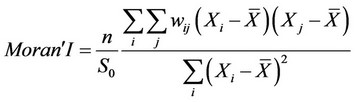
3.1.1. Globe Moran’ I Index Before our analysis, we usually assume that the agriculture economic activities have relationship in a certain region. This relationship distributes to goods price, information gap and so on. Also, the economic correlation shall have some kinds of geographical effect. How to measure this effect is reduced by location, and many researchers offer kinds of methods. But the popular and most acceptable method is Globe Moran’ I Index, which defined by:
where  and
and  denote observed value from region i and j, then
  and
and  are deviation of the variable of X in different regions with respect to the mean.
  is the average value of X;
  denotes a n space weight matrix, and be used to show the relationship between regions. The matrix
  is required because in order to address spatial autocorrelation and also model spatial interaction, we need to impose a structure to constrain the number of neighbors to be considered. There are two rules to establish the
  matrix: neighboring rule and distance rule, in this paper, we use the neighboring rule due to that each county has a clear boundary. The factor of diagonal in
  matrix is 0, and
 = 0 if region i neighboring to region j, otherwise,
  = 0.
= 0.
We can give the Z and P value to inspect the significance of Globe Moran’ I Index. Of course, it will automatically show in the result if calculating the Moran index using statistical software. In general, the significance level we selected is 0.05, on this level. If P value is less than this level, we can accept that the Moran’ I index shows a significant effect in the economic activities, otherwise, if P value is greater than the significance level, the effect showed by Moran’ I index is weakened.
3.1.2. Local Moran’ I Index and Local Indicator of Spatial Association The Globe Moran’ I index can tell us whether there is economic spatial autocorrelation in a certain region and the significance level through the Z value and P value. The analysis of globe Moran’ I index yields only one statistic to summarize the whole study area. In other words, global analysis assumes homogeneity. If that assumption does not hold, then having only one statistic does not make sense as the statistics should differ over spaces. Besides that, what we have more interest is the specific place if there is high correlation. The Local Moran’ I index can help us. The fact that Local Moran’s I is a summation of individual is exploited by the “Local Indicators of Spatial Association (LISA)” to evaluate the clustering in those individual units by calculating Local Moran’s I for each spatial unit and evaluating the statistical significance for each region. From the previous equation we then set the Local Moran’ I as following:

where n is the number of regions (observations). The other variables are the some with the globe Moran’ I index.
3.2. Theil Index
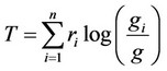
The Theil index is a statistic used to measure economic inequality. So, to see how the deferential in spatial regions, most traditionally, we can use Theil Index. The use of the dissimilarity Theil index to assess relative concentration is subject to a straightforward economic interpretation. In this paper, we will do some changes for the basic Theil index: separate the effect; we will discuss this in the next section. The basic Theil index formula is:
 denotes the proportion of population in region i,
  denotes the average output per person in region i.
4. DATA AND EMPIRICAL WORK
4.1. Data
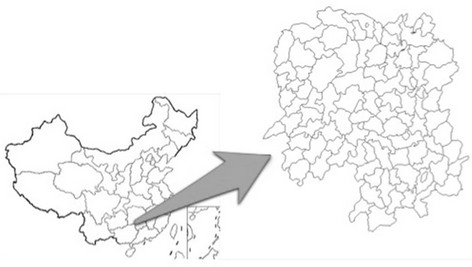
In this section, we consider the data that are available for studying the agriculture spatial distribution of economic activities. There are 31 provinces, 600+ cities and more than 2000 counties in China. As the basic unit, we choose county as the research unit due to their independent policy-making system. You can find a full economy structure in a single county: agriculture sector, industry sector, center city, etc. The county is a small integration economic system. The relevant notion of a basic region for this paper is the 88 counties in Hunan province area (See Figure 2), which locates on the south middle in China. There are 88 counties in Hunan province and these 88 counties are our data unit. These 88 unit counties cover over more than 95% of total land areas of Hunan province. The data we use is source from the public data from statistical book, it include: “Chinese county social and economic statistical year book” 2011, 2007 and 2000; “China Statistical Yearbook” 2011, 2007 and 2000; “China agricultural yearbook” 2011, 2007 and 2000. The data set used in this paper contains the main economic statistical data, such as population, total agriculture output, main agricultural products (Food, Meat, Cotton and Oilseed), of 88 counties in Hunan Province.
4.2. Agriculture Economic Distribution Pattern of Hunan Province
Figure 3 shows us a glance of distribution of total economic output of agriculture in Hunan province in 1999, 2006 and 2010. The top pic in the Figure 3 shows years’ total economic output bar chart (From left to right is 1999, 2006 and 2010). The agriculture output in 2010 doubles that in 1999, and also has a high increasing from 2006. The bottom pictures shows total agricultural economic output spatial location spread in Hunan on the corresponding periods (1999, 2006 and 2010). The distribution pattern is preformed as little cluster in west, northeast and mid-southwest. The increasing of produc-
 China
China
Figure 2. Hunan location and the county unit.
tivity in the high output areas is continuing to highly grow, and we can explain this phenomenon as the inner scale effect. High output areas trends to have higher output in next period due to the potential input of new resource and “Home Market Effect”. In high output areas, capital and technology skills have some kinds of advantage than other places, and we can call this advantage as “Advantage of Producer (AOP)”. AOP effect can be active only when there are abundant input factors, such as worker, land and nature resource.
The cluster pic at the bottom of Figure 3 shows us a change trend of agriculture economic output location that the form of agricultural spatial is from dispersing in northeast areas to clustering surrounding the triangle periphery circle gradually, which set by “Zhangjiajie-ChangshaShaoyang” as a city triangle shape (See the third pic at the bottom of Figure 3). It really presents some kind of agglomeration for agriculture outside the areas of cities in Hunan province. But the cluster level is slight and the agglomeration process is still going on. We can see little change of agriculture spatial location pattern from 2006 to 2010, but we also should notice that the cluster steps from 1999 to 2010 is obviously happening. The maps in
Figure 4 highlight the key stylized facts concerning the spatial distribution of four main agricultural products output across regions in Hunan province between 2006 and 2010, where from up to down are Food, Meat, Cotton and Oilseed.
The specific classification of agricultural products shows more significance in cluster and agglomeration in Hunan province. For Food, the output of Food products has a similar spatial location pattern with the total agriculture economic output location (See the first row pics in Figures 3 and 5). The similar spatial location pattern between Food and total output of agriculture contributed to high proportion of food supply of the whole agricultural products in Hunan. The Food supply presents a ring form spatial location pattern in the north of Hunan (See Figure 5). For Meat, the location pattern is more remote from the center and similar with Food. There also are some kinds of cluster for meat product in the southeast areas (See Figure 5). High productive area for meat clusters in the north and east of Hunan, but compared to the 2006, what differentiates with the food’s pattern is that most of counties with high productivity show some decline in output. The level of agglomeration for meat is
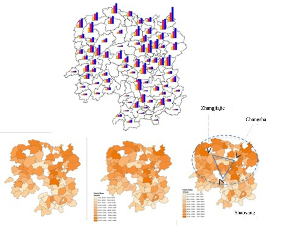
Figure 3. Hunan agricultural economic spatial location agglomeration and trends.

Figure 4. Local moran’ I index with LISA for agricultural output in Hunan province.
more obvious in 2006 than 2010.
The spatial location patterns of Cotton and Oilseed are more obvious (See Figure 5). There are high cluster patterns in the center of Hunan, which present a Line shape. Compared with that in 2006, the agglomeration level is more significant in 2010 for both Cotton and Oilseed.
The pattern of agriculture in Hunan, which shows that the spatial location cluster of agricultural products, characters with describing as exhibiting pattern of “Ring pattern in the north” for Food and Meat, “Line Pattern in the center” for Cotton and Oilseed (See Figure 5). The form of total agricultural output spatial is from dispersing in northeast areas to clustering surrounding the triangle periphery circle gradually, which is set by “Zhangjiajie-Changsha-Shaoyang” as a city triangle shape (See Figure 3). There is some evidence that this core-periphery pattern in agriculture economic output may be weakening among counties, while stable within counties.
In this case, Food and Meat follow a slight “Core-Periphery” pattern in Hunan, and we can figure it out on visual map. For Food, the wide core periphery pattern has more significance since 2006 as high output areas are more cluster. In contrast, the Meat core periphery pattern has some kind of declining slightly since 2006 as the high output areas are more dispersed. Cotton and Oilseed in Hunan province follow a clear pattern. We can identify a high output area for them and the line in center pattern in Hunan remained stable from 2006 to 2010.
4.3. The Relation Analysis of Agriculture Economic Spatial Location
In the previous section, we described the spatial loca-
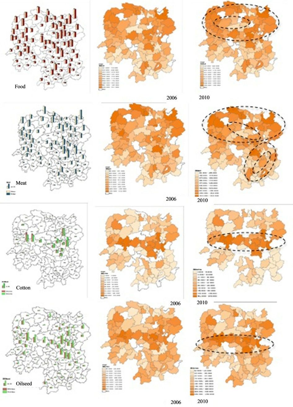
Figure 5. The spatial location for food, meat, cotton and oilseed in Hunan (up to low: food, meat, cotton, oilseed).
tion pattern for agriculture economic output and specify products (Food, Meat, Cotton and Oilseed) output by county level in Hunan. The problem emerges: are agriculture production areas having spatial autocorrelation in county level? Whether there are economic spatial autocorrelation in a certain region and how is their significance level? In this section, we will apply the spatial autocorrelation to identify tool to answer it. For the first question, whether the spatial autocorrelation exists, the Globe Moran’ I Index will be applied and for the following questions, whether there is a certain region with high cluster and how the significance level is, we will use the Local Moran’ I index. The fact that Local Moran’s I is a summation of individual is exploited by the “Local Indicators of Spatial Association (LISA)” to evaluate the clustering in those individual units by calculating Local Moran’s I for each spatial unit and evaluating the statistical significance for each region.
The Globe Moran’ I Index showed in the Table 1 presents the spatial autocorrelation level in 1999, 2006 and 2010 for total agriculture output, 2006 and 2010 for Food, Cotton, Meat and Oilseed by county level in Hunan province.
The conclusion of Table 1 summarizing the total agriculture output of county in Hunan shows some kind of spatial autocorrelation, even though the spatial autocorrelation is low, but stable from 1999 to 2010. Globe Moran’ I Index for total agriculture output are listed as 0.14, 0.11 and 0.13 in 1999, 2006 and 2010. The corresponding Z score and P value is Z(1.92), P(0.05); Z(1.72), P(0.08); Z(1.95), P(0.05). For total agricultural economic output, the significance set for Globe Moran’ I index presents more stable. The process of clustering total agriculture economic output is standing at slight agglomeration level (See Figure 6(b)).
The spatial autocorrelation of Cotton and Oilseed is higher than Food and Meat, and we can read the estimated result from Table 2. For the Cotton and Oilseed, the Globe Moran’ I index are 0.27 and 0.30 in 2006; 0.31 and 0.31 in 2010. The level of spatial autocorrelation is similar with each other between Cotton and Oilseed. We need to notice that the cotton’s spatial autocorrelation level shows some kind of increasing in 2010 compared to that in 2006. The Z score and P value to Globe Moran’ I Index for Cotton and Oilseed listed are: Z-cotton (3.83), P-cotton (0.00); Z-oilseed (4.47), P-oilseed (0.00) in 2006 and Z-cotton (3.90), P-cotton (0.00); Z-oilseed (4.71), P-oilseed (0.00) in 2010. The significance set for Globe Moran’ I index to Cotton and Oilseed presents higher in 2010 than that in 2006. The process of clustering for Cotton and Oilseed is getting to stronger agglomeration (Figure 4).
The spatial autocorrelation level of outputs for Food and Meat is slighter than Cotton and Oilseed, but it still presents positive effect in spatial autocorrelation. For the Food and Meat, the Globe Moran’ I index are 0.12 and 0.13 in 2006; 0.13 and 0.16 in 2010, which shows some kind of increasing in the digital level from 2006 to 2010. The level of spatial autocorrelation is similar with each other between Food and Meat. The Z score and P value to Globe Moran’ I Index for Food and Meat listed are: Z-food (1.90), P-food (0.06); Z-meat (2.02), P-meat (0.04) in 2006 and Z-food (1.93), P-food (0.05); Z-meat
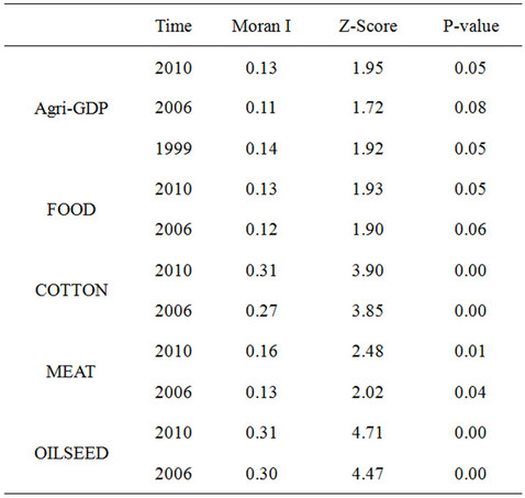
Table 1. The globe Moran’ I index for agriculture output of county in Hunan Province.
 (a) (b)
Figure 6. Spatial autocorrelation and cluster level.
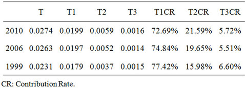
Table 2. Theil index: Decomposition effect of population structure.
(2.48), P-meat (0.01) in 2010. Similar to Cotton and Oilseed, the significance set for Globe Moran’ I index to Food and Meat presents higher in 2010 than 2006. The process of cluster for Food and Meat is getting to slight agglomeration and getting to higher in future.
The analysis of globe Moran’ I index yields only the statistics to summarize the whole area spatial autocorrelation level in Hunan. But what we are more interest is the specific place if there is high correlation for agriculture output. In this section, we will apply the Local Moran’ I index tool exploited by the “Local indicators of spatial association (LISA)” to evaluate the clustering in those individual county units by calculating for each county unit and evaluating the statistical significance. Figure 6 is mapping the result of estimate of Local Moran’ I Index with LISA method.
The three top maps in the Figure 6 show the local cluster effect for total agricultural economic output in Hunan province by county unit. It present the high output of agriculture locates in center and northeast. The dark area in the map means there are high output and also high output area surrounding it. There is positive scale effect for high output of total agriculture. Also, these high product positive scale effect areas are slight declining from 1999 to 2010 (See Figure 6). The high output areas with high spatial autocorrelation for agriculture in Hunan are locating surrounding the Changsha city (In the northeast of Hunan) and Shaoyang city (In the center near to southwest of Hunan), this phenomenon presents the significant effect from city development for agriculture development. We can notice that the High output hotpot areas are relative to “Peri-urban zones”. The bottom maps summarize the four main products (Food, Meat, Cotton and Oilseed) output local cluster effect and the comparable between 2006 and 2010. Food and Meat have similar distribution of local cluster effect, and it show this effect is weaken in the south more than in the north. Especially for meat output, the high output areas spatial correlation in the south is weaken in 2010 than it in 2006. In contract, cotton and oilseed show a different side. The high output areas effect of cotton and oilseed are higher in 2010 than 2006 and we can image this process still be continue, especially for oilseed (See Figure 6). We can set this phenomenon for cotton and oilseed as high output spillover effect.
For the low spatial output effect areas, the low output can’t be change even thought there are high output areas surrounding it. This may be cause by lack of agriculture resource, such as water, land or insufficient on worker and so on. These areas can be set as “poor natural resources” in Table 1. On the other hand, the low product of agriculture may be cause by the land be occupy for other using, especially for tourism, these areas can be set as “the middle countryside” or “remote rural areas” in Table 1. Theoretically, for the explaining of phenomenon of agriculture distribution pattern can be focused mainly on the role of demand externalities in determining agricultural locations. In particular, do not like the industrial agglomeration, the types of demand externalities that induce agriculture cluster are often set just only for one certain agriculture products, but for some product, there still exist their spatial market overlap between neighbor regions. In such case, it’s natural for those agriculture products show some kind of “ring pattern” surrounding the marketplace. More over, in terms of nature environment and transportation situation, it is also natural for agglomerations in certain place as more concentrated to coincide with those of less concentrated, and leading to the type of synchronization predicated by the hierarchy principle.
4.4. Spatial Inequality Measured by Theil Index
Obviously, the agriculture output show significant gap between counties in Hunan province, the analysis of location pattern in previous can prove this. In this settion, we will apply the Theil Index to analysis the inequality of agriculture product in Hunan province. What we focus on is worker efficient and the structure of population. After this work, we need to decomposition the Theil Index with population style.
The Theil index is a statistic used to measure economic inequality. It can help us to figure out the factor and their contribution for inequality (See the original Theil Index formula in section 3). We split the Theil Index according the deviation of human factor: R. We divided population R to three overlap part: agricultural employed population: , rural population:
 , and total population:
 . The relationship of them is:
  (See Figure 7). Then for the average agriculture output per per-son
  can be divided as
 , where
  denotes labor productivity for agriculture output,
  denotes the agriculture employed rate and
  denotes the agriculture population proportion. So we can reset the

Figure 7. The relationship of population structure.
Theil Index as:
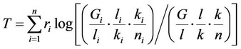
Decomposed to:

And we can set:

So:
The previous section considers the agriculture economic spatial location pattern by using county data in Hunan province, the pattern map show us directly that there exist some kind of differentials among different counties. The Theil Index for counties agricultural output show that the inequality between 88 counties in Hunan is increasing slightly from 1999 to 2010. The total Theil Index list as: T1999(0.0231), T2006(0.0263) and T2010(0.0274). The reason for inequality are very complex, in this paper, we take our focuses on the cause from person. From the Table 2, it seems that the labor productivity is the biggest cause the agricultural economic inequality between counties in Hunan province, the contribution rate of labor productivity to those inequality is more than 70%. But the influence of labor productivity to agricultural shows a declining during 1999 to 2010. The agriculture employed rate show a increasing influence to the agricultural inequality between regions. From 1999 to 2010, the agriculture employed rate contribution rates to agricultural inequality between 88 counties in Hunan are list as: 15.98%, 19.65% and 21.59%. The agriculture population proportion do some kind of contribution to the regional agricultural inequality, the influence to agricultural output inequality in Hunan is stable (See Table 2).
5. CONCLUSIONS
This paper provides an empirical work for agriculture spatial distribution and considers what we know about the spatial location pattern in order to offer spatial views on the agriculture economic research. Also, we know that the periphery areas exist significant differential among regions. Set county as basic unit to analysis shows us that: It really presents some kind of agglomeration for agriculture outside the areas of city in Hunan province; The pattern of agriculture in Hunan shows that the spatial location cluster of agriculture products characters with describing as exhibiting pattern of “Ring pattern in the north” for Food and meat, “Line Pattern in the center” for cotton and oilseed. In additional, for total agricultural economic output, the significance set for Globe Moran’ I index are presents more stable. The process of cluster agricultural economic total output is standing at slight agglomeration level. The process of cluster for cotton and oilseed is getting to more strong agglomeration and food and meat is getting to slight agglomeration and getting a process to higher in future. Theil Index result shows us the labor productivity is the biggest cause the agricultural economic inequality between counties in Hunan province.
We have to accept that many economists take their emphasis on industrial sector, especially for the economic geography, many researches neglected to study the role of agricultural sector in the process of cluster and how the agriculture sector agglomeration by itself. We can jump out agriculture to analysis the whole economic or even only a city, still, agriculture take an important part f the economy in most developing country, like China, and it seems that the cluster of agriculture has give some significant phenomenon in those areas. In additional, developing countries agriculture is often subject to important policy issues.
6. ACKNOWLEDGEMENTS
The research works for this paper was supported by the National Philosophy and Social Science Foundation of China (No. 11 & ZD009).
REFERENCES
- Brülhart, M. (1998) Economic geography, industry location, and trade: The evidence. The World Economy, 21, 775-801. doi:10.1111/1467-9701.00163
- De Lucio, J., Herce, J. and Goicolea, A. (2002) The effects of externalities on productivity growth in Spanish industry. Regional Science and Urban Economics, 32, 241- 258. doi:10.1016/S0166-0462(01)00081-3
- Venables, A.J. (1996) Equilibrium locations of vertically linked industries. International Economic Review, 37, 341- 359. doi:10.2307/2527327
- Fujita, M., Krugman, P. and Venables, A. (1999) The spatial economy. MIT Press, Cambridge.
- Fujita, M. and Thisse (2002) Economics of agglomeration: Cities, industrial location, and regional growth. Cambridge University Press, Cambridge.
- Fujita, M. and Thisse, J.F. (2002) Economics of agglomeration: Cities, industial location, and regional growth. Cambridge University Press, Cambridge.
- Gruber, S. and Soci, A. (2010), Agglomeration, agriculture, and the perspective of the periphery. Spatial Economic Analysis, 5. doi:10.1080/17421770903511353
- Ottaviano, G.I.P. and Puga, D. (1998) Agglomeration in the global economy: A survey of the new economic geography. World Economy, 21, 707-731. doi:10.1111/1467-9701.00160
- Ottaviano, G.I.P. and Robert-Nicoud, F. (2006) The “genome” of NEG models with vertical linkages: A positive and normative synthesis. Journal of Economic Geography, 6, 113-139. doi:10.1093/jeg/lbh070
- Hanson, G.H. (2001) Scale economies and the geographic concentration of industry. Journal of Economic Geography, 1, 255-276. doi:10.1093/jeg/1.3.255
- Wiggins, S. and Proctor, S. (2001) How special are rural areas? The economic implications of location for rural development. Development Policy Review, 19, 427-436. doi:10.1111/1467-7679.00142
- Baldwin, R.E. (2001) Core-periphery model with forwardlooking expectations. Regional Science and Urban Economics, 31, 21-49. doi:10.1016/S0166-0462(00)00068-5
- Bosker, M., Brakman, S., Garretsen, H. and Schramm, M. (2007) Looking for multiple equilibria when geography matters: German city growth and the WWII shock. Journal of Urban Economics, 61, 152-169. doi:10.1016/j.jue.2006.07.001
- Chan, K.W. (1994) Urbanization and rural-urban migration in China since 1982: A new baseline. Modern China, 20, 243-328. doi:10.1177/009770049402000301
- Duranton, G. and Overman, H. (2005) Testing for localisation using micro-geographic data. Review of Economic Studies, 72, 1077-1106. doi:10.1111/0034-6527.00362