Low Carbon Economy
Vol. 3 No. 3A (2012) , Article ID: 25022 , 4 pages DOI:10.4236/lce.2012.323013
An Econometric Analysis for CO2 Emissions, Energy Consumption, Economic Growth, Foreign Trade and Urbanization of Japan
![]()
Department of Accounting and Information Systems, Faculty of Business Studies, University of Dhaka, Dhaka, Bangladesh.
Email: sharif_hossain04@yahoo.com
Received September 7th, 2012; revised October 10th, 2012; accepted October 21st, 2012
Keywords: Dynamic Causal Relationship; ADF and PP Tests; ADRL Bound Test; VEC Model
ABSTRACT
This paper examines the dynamic causal relationship between carbon dioxide emissions, energy consumption, economic growth, foreign trade and urbanization using time series data for the period of 1960-2009. Short-run unidirectional causalities are found from energy consumption and trade openness to carbon dioxide emissions, from trade openness to energy consumption, from carbon dioxide emissions to economic growth, and from economic growth to trade openness. The test results also support the evidence of existence of long-run relationship among the variables in the form of Equation (1) which also conform the results of bounds and Johansen conintegration tests. It is found that over time higher energy consumption in Japan gives rise to more carbon dioxide emissions as a result the environment will be polluted more. But in respect of economic growth, trade openness and urbanization the environmental quality is found to be normal good in the long-run.
1. Introduction
In the last three decades the increase in greenhouse gases emissions is a major threat of global warming and climate change has been the major on-going concern for all societies from developing countries to developed countries. The economic growth of the developed countries impels intensive use of energy and other natural resources and as a result more residues and wastes are throwing in the nature that could lead to environmental degradation. Carbon dioxide (CO2) is regarded to be the main source of green house effect and has captured great attention in recent years. Most of the CO2 emissions come from fossil fuels consumption such as coal, oil and gas, the main power of source of automobile and industry that are directly linked with economic growth and developments.
In 2007, the Intergovernmental panel on Climate Change (IPCC) report reveals that at the present time total annual emissions of GHGs are rising. Over the last three decades, GHG emissions have increased by an average of 1.6% per year1 with carbon dioxide (CO2) emissions from the use of fossil fuels growing at a rate of 1.9% per year.
In the absence of additional policy actions, these emission trends are expected to be continued.
It is projected that with current policy setting global energy demand and associated supply patterns based on fossil fuels, the main drivers of GHG emissions will continue to grow. Atmospheric CO2 concentrations have increased by almost 100 ppm in comparison to its preindustrial level, reaching 379 ppm in 2005, with mean annual growth rates in the 2000-2005 period that were higher than those in the 1990s. The total CO2 equivalent (CO2) concentration of all long-lived GHGs is currently estimated to be about 455 ppm CO2, although the effect of aerosols, other air pollutants and land-use change reduces the net effect to levels ranging from 311 to 435 ppm CO2 (high agreement, much evidence (IPCC (2007)). Despite continuous improvements in energy intensities, global energy use and supply are projected to continue to grow, especially as developing countries pursue industrialization.
Should there be no substantial change in energy policies, the energy mix supplied to run the global economy in the 2025-2030 time frame will essentially remain unchanged more than 80% of the energy supply will be based on fossil fuels, with consequent implications for GHG emissions. On this basis, the projected emissions of energy-related CO2 in 2030 are 40% - 110% higher than in 2000, although per capita emissions in developed countries will remain substantially higher (IPCC (2007)). For 2030, GHG emission projections (Kyoto gases) consistently show a 25% - 90% increase compared to 2000, with more recent projections being higher than earlier ones (high agreement, much evidence).
Global climate change threatens to condemn millions of people to poverty. Millions of people in each and every year of developed nations to least developed nations are suffering from climate change disasters like as floods, cyclones, droughts, tsunamis etc. It is predicted that the effects of global warming will lead to the rise of sea level by 20 feet by 2020, threatening coastal areas with floods. If the global temperature rise of between 3 to 4 degrees Celsius would displace 340 million people through flooding, droughts would diminish farm output, and retreating glaciers would cut drinking water from as many as 1.8 million people.
The UN report of 2007 says that if in the next 15 years follow the same trend as the past 15 years, the dangerous climate change will become unavoidable. To avoid catastrophic impact, the rise in global temperature must be limited to 2 degrees Celsius. But emissions from cars, power plants and serve deforestation in Brazil, Indonesia and elsewhere are twice the level need to meet that target. The increasing volume of CO2 emissions due to expanding and widening of the process of industrialization and the consequent of urbanizations all over the world are the determinant factors of the ascending greenhouse threats. Therefore the research of this aspect becoming more importance for all societies from developing countries to developed countries.
Since 1990s, the researchers intensively assessed the impacts of global warming on the world economy. The most popular word-wide organizations, such as United Nations have been attempting to reduce the adverse impacts of global warming through intergovernmental and binding agreements. The Kyoto protocol that was signed in 1997 to the United Nations Framework Convention on Climate Change (UFCCC) with the objective of reducing the greenhouse gases (GHG) which causes rise to warmer global temperature. The Kyoto protocol determined the constraints to environmental pollutants are requires a timetable to realize the reduction of GHG emissions of the developed countries. It demands the reduction of GHG emissions to 5.2% during 2008-2012 which is lower than 1990. The Japan is one of the member countries of Kyoto protocol and gave a commitment to reduce GHG emissions by 6% for 2012 with reduction of emissions from consumption of fossil fuels by 16%. Still now, most of the countries are failure to fulfill their commitment including Japan. Japan is taking major steps to reduce the carbon dioxide emissions from the consumption of fossil fuels. The amount of carbon dioxide emissions of Japan over a period of times after Kyoto protocol is represented by the following Figure 1.
From this figure it seems that in recent years the carbon emissions from energy consumption are declining very rapidly. Thus a general question can be raised in our mind, due to reduction of carbon dioxide emissions whether economic growth will be affected in Japan. That is why to given the answer of this question in this paper the principal purpose has been made to investigate the dynamic causal relationship between carbon dioxide emissions, energy consumption, economic growth, foreign trade and urbanization of Japan using time series data for the period of 1960 to 2009. Also another attempt has been made to investigate the Narayan and Narayan [1] approach for the time series data of Japan. The organizational structure of this paper is as follows: Section 2 reviews related literature; Section 3 discusses data sources and some descriptive statistics; Section 4 provides empirical model and conceptual framework for this study; Section 5 discusses econometric modeling framework with empirical analysis and Section 6 concludes with a summary of the main findings and policy implications.
2. Literature Review
In respect of empirically examine the relationship between economic growth, energy consumption and carbon emission which is considered as a proxy variable for environmental quality (Soytas and Sari [2]), there has been basically three research strands. The first strand of research focuses on the environmental pollutants and economic growth nexus. The literature on environmental quality and economic growth study mainly focuses on the testing of the existence of environmental Kuznet’s curve (EKC). In this context, Grossman and Krueger [3] along with Shafiq [4], Dinda and Coondoo [5], Heil and Selden [6], Friedl and Getzner [7] attempted to test the existence of EKC for different economies. The results of
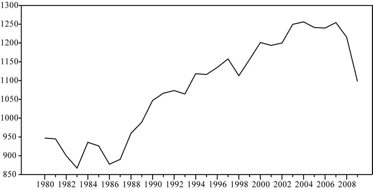
Figure 1. Amount of carbon dioxide emissions from consumption of energy over a period of time; Source: International Energy Statistics; Units are given in million tones.
such research are however contradictory and in many cases researchers failed to establish the inverted U relationship with real life data. A similar yet detailed branch of research attempts to analyze the link between energy consumption and output, suggesting that economic development and output may be jointly determined and the direction of causality between these two variables needs to be tested. Following the seminal work of Kraft and Kraft [8], several others including Masih and Masih [9], Yang [10], Wolde-Rufael [11], Narayan and Singh [12], Narayan and Russell [13] tested the energy consumption and economic growth nexus with a variety of techniques and for different panel of countries. The recent studies in the area of growth-pollution-energy consumption nexus however attempt to link these two branches of literatures while combining them in a single multivariate framework. Ang [14], Soytas, Sari and Ewing [15], Halicioglu [16], Tamazian and Rao [17] initiated this combined line of research. Among the recent literature involving the testing of EKC, Lean and Smyth [18] found non-linear relationship between emission and real output. The finding of Akbostanci, Turut-Asik and Tunc [19] on Turkish economy was however different from that of Lean and Smyth [18] as the former found an increasing relationship between carbon emissions and income in the long run when they looked at cointegration between carbon emissions and per capita income for Turkish economy. Their panel time series analysis of 58 provinces of Turkey on the contrary, revealed an N-shaped relationship for SO2 and PM10 (two pollutants commonly referred in connection to air pollution). He and Richard (2010), while using 57 years of data for Canadian economy also found no strong evidence of EKC. The findings of Tamazian and Rao [17] on the other hand provided an optimistic picture as they found economic and financial development helping to reduce environmental degradation of BRIC countries.
Despite enormous amounts of literature on energy and output, the second strand of the research mainly focuses on studies that examine the causal relationships between energy consumption and output growth, particularly in developing countries. The studies that find no causality between energy consumption and income in the US include those by Akarca and Long [20], Yu and Hwang [21], Stern [22], and Cheng [23]. The same result is true for the U.K. Yu and Choi [24] and France, Erol and Yu [25]. Studies that find two-way causation are in South Korea include those of Masih and Masih [26], Glasure [27], and Oh and Lee [28]. A similar causation for Philippines and Thailand is found by Asafu and Adjaye [29]. Unidirectional causation from output to energy consumption is found in countries like Australia; Narayan and Smyth [30], India; Cheng [31], Singapore; Chang and Wong [32], Glasure and Lee [33], South Korea; Soytas and Sari [34], and Taiwan; Cheng and Lai [35]. A number of studies have found the direction of causality from energy consumption to output growth.2
In addition, researchers have attempted to incorporate not only output/income or economic development per se but also extended their analysis for financial development or for variables capturing openness or trade intensity of a country. The study of Grossman and Krueger [36] is pioneering in this regard. In recent years, Halicioglu [16] while using Turkish data also incorporated trade into the framework of CO2 emission, income and energy consumption. Their analysis revealed that, for Turkish economy income is the most crucial determinant of carbon emission, followed by energy consumption and finally it is trade. They found two types of relationship among these variables, where one type of relation revealed that CO2 emission is determined by not only energy consumption and income but also through trade. The second type of relationship showed that carbon emission, energy consumption along with foreign trade, all play important role in determining the level of income of Turkey. The importance of foreign trade in determining the level of CO2 emission has also been emphasized by Anderson, Quigley and Wilhelmsson [37]. In their analysis, while attempting to analyze the emission generated in the transport sector, they concentrated on the export of China and found that trade play important role in generating emission in transport sector and greater emission is attributable by exports than by imports.
Finally, a third stream of research has emerged, which combines earlier two approaches by examining dynamic relationship between carbon emissions, energy consumption and economic growth. Soytas, Sari and Ewing [15] investigate energy consumption, output and carbon emission nexus for USA using augmented vector auto regression (VAR) approach of Toda and Yamamoto [38] after incorporating gross fixed capital formation and labor force into the model. They found non-causality between income and carbon emission and between energy use and income. However, the study found unidirectional Granger causality running from energy consumption to carbon emission. Using the same approaches and variables, Soytas and Sari [39] found same link between income and carbon emission in Turkey though the study establishes unidirectional Granger causality from carbon emission to energy consumption in long run. So both USA and Turkey can reduce their carbon emissions without forgoing economic growth. Zhang and Cheng [40], using the Toda and Yamamoto [37] procedure, investigate the energy consumption, output and carbon emission nexus for China, controlling for capital and urban population. They found unidirectional long-run causality running from GDP to energy consumption and from energy consumption to carbon emission. The study showed that neither carbon emission nor energy consumption leads economic growth. Sari and Soytas [41] investigate the relationship between carbon emissions, income, energy and total employment in five OPEC countries by employing the autoregressive distributed lag (ARDL) model of cointegration. Cointegration among the variables has been established only in Saudi Arabia. The study established that none of these countries namely Algeria, Indonesia, Nigeria, Saudi Arabia and Venezuela need to sacrifice economic growth in order to reduce CO2 emissions. Halicioglu [16], applying ARDL approach of cointegration in a log linear quadratic equation between per capita CO2 emission, per capita energy use, per capita real income, square of per capita real income and openness ratio, finds that there is a short-and long-run bi-directional causality between carbon emission and income in Turkey. In a similar kind of study, Jalil and Mahmud [42] found unidirectional causality from economic growth to CO2 emission in China. The study also indicates that the carbon emissions are mainly determined by income and energy consumption in the long-run. Trade has a positive but statistically insignificant impact on CO2 emissions. Amongst others, Tamazian and Rao [17] conducted detailed analysis on financial development-environment nexus and included variables like stock market value added, foreign direct investment, deposit money bank assets, capital account convertibility, financial liberalization, financial openness etc. to capture the level of financial development. Here, the authors also included conventional variables e.g. GDP and GDP-squared along with variables reflecting industrial development and level of research and development of a country where the later group of variables embodied economic development from a broader perspective. In terms of the effect of financial development on environmental quality their analysis offered interesting findings as financial liberalization and financial openness were found to be essential for reducing the emission of CO2. In addition, they also found capital market, banking sector development, greater flow of FDI all acting as positive factors to lower per capita CO2 emissions. Over time the research on environment-development nexus has not only extended and modified in terms of the research questions addressed, but also has developed from the view point of methodology and econometric modeling techniques. Most of the studies like that of Akbostanci, Turuk-Asik and Tunc [19] have applied cointegration technique and Granger causality method to understand the nexus. In terms of the findings of these analyses, no clear cut conclusion can be made and results differ depending upon the variables used and countries considered. In this context, a recent study conducted by Lean and Smyth [18] with panel data attempted to examine the long-run relationship between CO2 emissions, electricity consumption and output as well as the causal relationship between these variables. Their analysis revealed that there is short-run panel Granger causality from carbon emission to electricity consumption and long-run unidirectional causality from electricity consumption and CO2 emission to GDP. Akbostanci Turuk-Asik and Tunc [19] also find pollution and income variables being cointegrated. In addition to the above mentioned methodology of cointegration, He and Richard [26] adopted a wide range of techniques to understand the relationship between emission and economic/financial development. For example, they considered that the traditional parametric methodology of estimating EKC is not a flexible way to estimate the relationship and rather used semi parametric and flexible non linear parametric modeling.
According to the knowledge of the author, still now no one incorporated the variables foreign trade and urbanization in determining the level of carbon dioxide emissions in case of Japan. In Japan due to economic development, rural population is migrated in urban area, as a result urban populations pressure on urban resources and environment, thus environment is polluted. Thus to know the impact of urbanization (% of urban population of total) on pollution whether it is significant or not, is considered for this empirical study. Thus this paper shall fill the gap in the literature of the relationship between economic growth, energy consumption and carbon emissions by studying the dynamic causal relationship between carbon dioxide emissions, energy consumption, economic growth, trade openness and urbanization of Japan.
3. Data Sources and Descriptive Statistics
Annual data for CO2 emissions (CO2) (metric tons per capita), energy consumption (EN) (kg of oil equivalent per capita), per capita real GDP (PGDP) (constant 2000 US $) which is used as the proxy of economic growth, trade openness (OPEN) (% of exports and imports of GDP) which is used as the proxy of foreign trade, and urbanization (UR) (% of urban population of total) are downloaded from the World Bank’s Development Indicators. The data is for the period from 1960 to 2009. The descriptive statistics mean, standard deviation (Std. Dev.) and coefficient of variation (CV) of these variables are recorded below in Table 1.
From the reported values in Table 1, it is found that
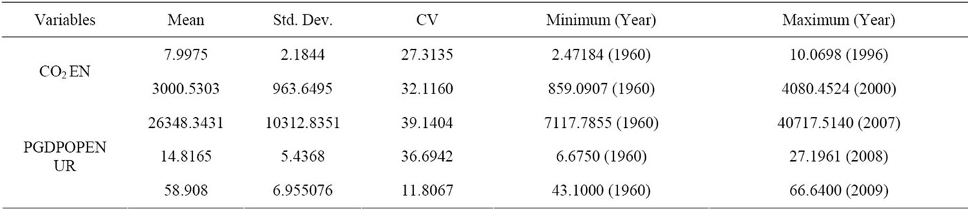
Table 1. Descriptive statistics for different variables.
variability is highest for the variable economic growth and lowest for urbanization.
4. Empirical Model and Conceptual Framework
4.1. Empirical Model
In order to find the long-run relationship between CO2 emissions, energy consumption, economic growth, foreign trade and urbanization, the following linear logarithmic form is proposed
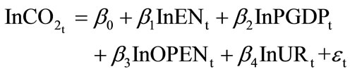 (1)
(1)
where CO2 is carbon dioxide emissions per capita, EN is energy consumption per capita, PGDP is per capita real GDP, OPEN is trade openness, UR is urbanization and ε is the random error term. The parameters  and
and  represent long-run elasticity of carbon dioxide emissions with respect to EN, PGDP, OPEN and UR respectively.
4.2. Conceptual Framework
The burning of fossil fuels to produce industrial goods in Japan is growing in recent years. While it is true that burning of fossil fuels emits a high amount of CO2 and pollutes our environment. It is empirically and theoretically shown that an increase in energy consumption results in greater economic activity. Thus we can expect that energy consumption and high level of economic growth (GDP) have positive impact on CO2 emissions at least in the short run. Thus from Equation (1) we have α1 > 0 and α2 > 0. International trade causes the movement of produced goods from one country to another for either consumption or for further processing. More consumption of goods and further processing of goods, which takes place due to greater trade openness, is a source of pollution. This implies that pollution is stimulated from further process and manufacturing of goods which results from greater trade openness. Thus we can expect that the variable trade openness has a positive impact on CO2
emission indicates that α3 > 0 in Equation (1) at least in the short-run. Finally in case of urbanization most cities are growing at a faster rate than the national average, as the endurance workers are migrating from rural area to urban area for better jobs, better life, better education, better treatment, etc. Thus urban populations pressure on urban resources and environment as a result environment is polluted. Thus we expect that there is a positive impact of urbanization on CO2 emissions, indicates that α4 > 0 in Equation (1). But the expectations of signs of the coefficients of Equation (1) based on subjective judgment are not always true, in reality. That is why, in this study the variables energy consumption, economic growth, trade openness and urbanizations are introduced in the model in determining the level of carbon dioxide emissions for Japan.
5. Econometric Methodology
On the basis of modern econometrics techniques, the dynamic causal relationship between carbon emissions, energy consumption, economic growth, trade openness and urbanizations has been examined in this paper. The testing procedure involves the following steps. At the first step whether each variable contains a unit root has been examined. If the variables contain a unit root, the second step is to test whether there is a long run-cointegration relationship between the variables. If a long-run relationship between the variables is found, the final step is estimate vector error correction model in order to infer the Granger causal relationship between the variables. The long-run and short-run elasticities of carbon emissions with respect to EN, PGDP, OPEN and UR have been calculated using the GMM method.
5.1. Unit Root Tests
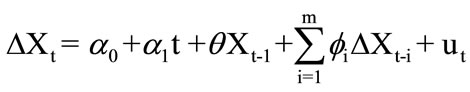
It is well known that the usual techniques of regression analysis can result in highly misleading conclusion when variables contains stochastic trend; Stock and Watson [43], Granger and Newbold [44]. In particular if the dependent variable and at least one independent variable contain stochastic trend, and if they are not cointegratedthe regression results are spurious; Phillips [45], Granger and Newbold (44). To identify the correct specification of the model, an investigation of the presence of stochastic trend in the variables is needed. The Augmented Dickey-Fuller (ADF) [46] and the Phillips-Perron (PP) [47] tests are applied in order to investigate that each of the variables contains stochastic trend or not. The estimation technique of these two tests is described below;
 . (2)
. (2)
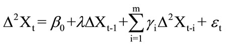
Here Xt is the series under investigation, Δ stands for first difference and the lagged difference terms on the right hand side of the equations are designed to correct for serial correlations of the disturbance terms. The lagged differences are selected by using AIC and SBIC criteria. If θ = 0, the series Xt contains a unit root and therefore an I(1) process governed by a stochastic trend. If a time series variable is integrated of order one, we have to investigate the 2nd order unit root and the equation is given by;
 (3)
(3)
where Δ2 is the second-difference operator. If λ = 0, the series Xt is said to be integrated of order two (I(2)). Let d represents the number of times that Xt needs to be differenced in order to reach the stationary. In this case Xt is said to be integrated of order d and is denoted by I(d). Since the estimated θ does not have the usual asymptotic distribution, the values tabulated by MacKinnon [48] are used. The Augmented Dickey Fuller [46] and the Philips-Perron [47] tests results are given below in Table 2.
From the ADF and PP tests results, it can be said that the variables carbon dioxide emissions, energy consumptions and trade openness are integrated order (1) and the variables economic growth and urbanization are integrated of order two.
5.2. Bounds Test Approach for Cointegration
The bounds test approach for cointegration, known as the autoregressive-distributed lag (ARDL) of Pesaran Shin and Smith [49], has become most popular amongst researchers. The bounds test approach has certain econometric advantages in comparison to other single equation cointegration procedure. They are as follows: 1) endogeneity problems and inability to test hypotheses on the estimated coefficients in the long-run associated with
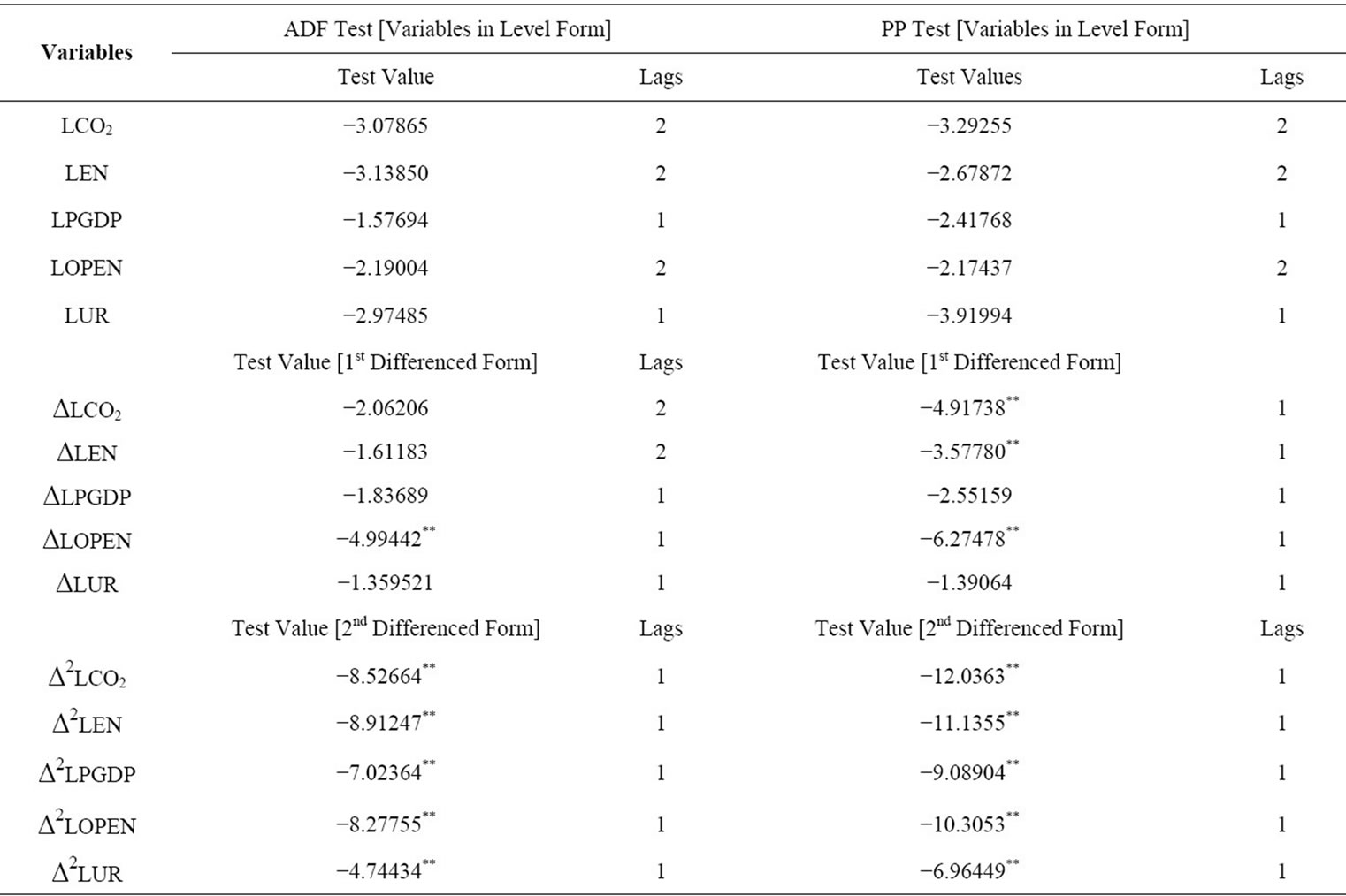
Table 2. The Augmented Dickey-Fuller (ADF) and Philips-Perron (PP) tests results.
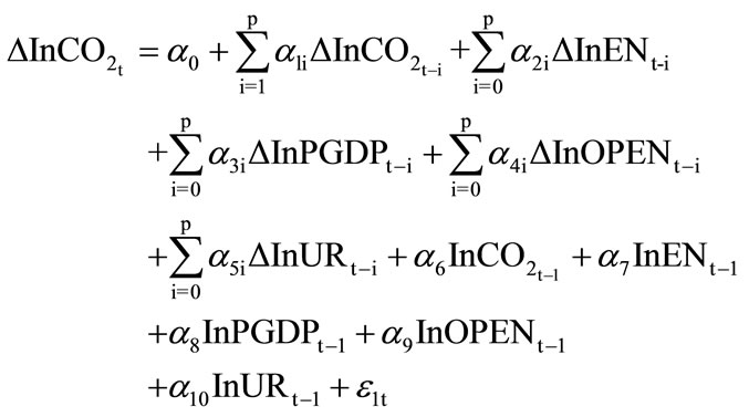
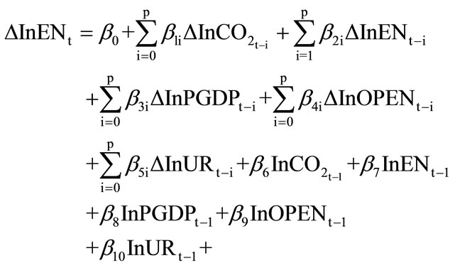
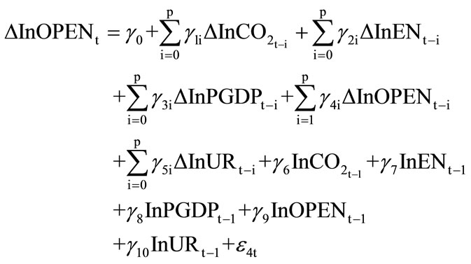
the Engle-Granger method, are avoided; 2) the long-run and short-run parameters of the model in question are estimated simultaneously; 3) the bounds test approach for testing the existence of long-run relationship between the variables in levels is applicable irrespective of whether the underlying time series variables are purely I(0), I(1) or fractionally integrated; 4) the small sample properties of the bounds testing approach are far superior to that of multivariate. In this paper to implement the bounds test for cointegration, the following unrestricted regression equations have been formulated:
 (4)
(4)
 (5)
(5)
 (6)
(6)
 (7)
(7)
 (8)
(8)
According to Pesaran, Shin and Smith [49], the joint F-test of the lagged level variables in Equations (4)-(8) are used to test the presence of long-run equilibrium relationship. For instance in Equation (4) the test for cointegration is carried out by testing the null hypothesis of no conintegration is defined by H0: α6 = α7 = α8 = α9 = α10 = 0, using the F-test. The variables are said to be cointegrated if the null hypothesis of no cointegration is rejected; otherwise the variables are not cointegrated. Similarly, procedures can also be carried out for testing the long-run equilibrium relationships for Equations (5)-(8).
The asymptotic distribution of the F-statistic is nonstandard under null hypothesis and it was originally derived and tabulated by Pesaran, Shin and Smith [49]. Two sets of critical values are provided; one which is appropriate where all the series are I(0) and the other is appropriate where all the variables are I(1). According to Pesaran, Shin and Smith [49], if the calculated F-statistic falls above the upper critical value, a conclusive inference can be made regarding cointegration without knowing whether the series are I(0) or I(1). In this case the variables are said to be cointegrated indicates existence of long-run relationship among the variables. Alternatively if the calculated F-statistic falls below the lower critical value the null hypothesis of no cointegration will not be rejected regardless whether the series are I(0) or I(1). In contrast the inference is inconclusive if the calculated F-statistic falls within lower and upper critical values unless we know whether the series are I(0) or (1). The estimated results are given below in Table 3.
The critical value ranges of F-statistic are 4.614 - 5.966, 3.272 - 4.306 and 2.676 - 3.586 at 1%, 5% and 10% level of significance respectively.
From the estimated results it can be concluded that there exits three cointegration relationships. The first long-run relationship refers to the situation where lnCO2 is the dependent variable and the second long-run relationship refers to the situation where lnEN is the dependent variable and third long-run relationship refers to the situation where lnPGDP is the dependent variable. The results are inconclusive where lnOPEN and lnUR are the dependent variables.
To investigate the robustness of ARDL bounds test
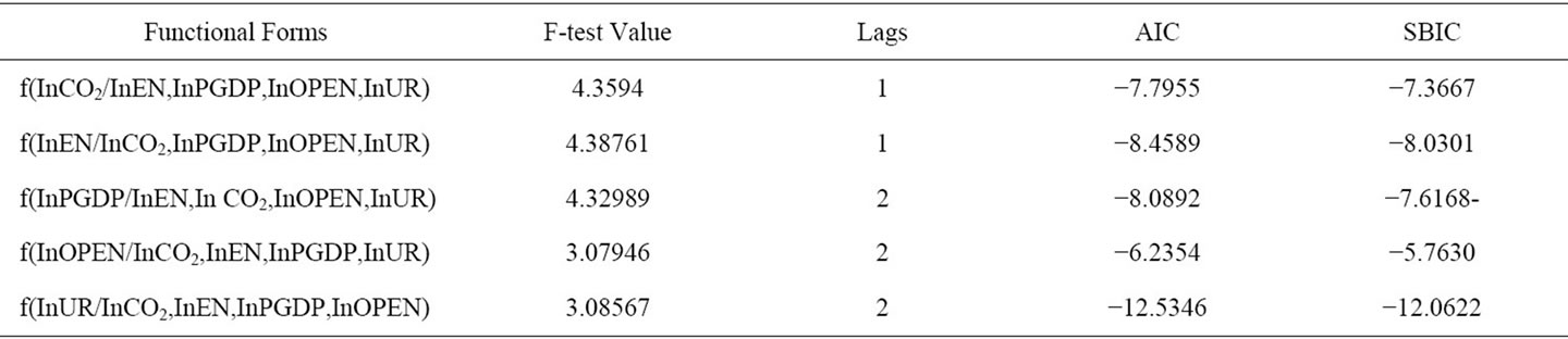
Table 3. The results of F-test for cointegration relationship.
approach for long-run relationship, I also applied the Johansen and Juselius’s [50], test. Since the Johansen and Juselius’s [50] multivariate cointegration methodology is fairly well documented, a brief reminder of this method is given below
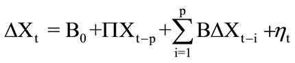 (9)
(9)
where Xt represents a vector of endogenous I(1) variables, B0 represents a vector of constant terms, B is a matrix of coefficients, ηt is a vector of residuals, and p denotes the lag length. All variables in Equation (9) are deemed to be potentially endogenous. The long-run equilibrium relationship among Xt is determined by the rank of P (say r). If r is zero, the variables in level form do not have any cointegration relationship and the Equation (9) can be transformed to VAR model of pth order. If 0 < r < n, then there are n × r matrices of α and β such that
 . (10)
The strength of cointegration relationship is measured by α, β is called cointegration vector and β’Xt is I(0) although Xt are I(1). The cointegrating rank can be found via the trace and the maximum eigenvalue tests. The lag length of the unrestricted vector autoregressive (VAR) model in Equation (10) is determined on the basis of AIC and SBIC criteria and the adjusted likelihood ratio (LR) test is most commonly used. The test results are reported below in Table 4.
The trace test and the maximum eigen value test results indicate that there exist three cointegration equations. Since, it has been found that there exists a cointegration vector among the variables, the following cointegration model is projected here,
 (11)
(11)
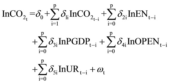
The selection of the orders of lags in the ARDL models is very sensitive which is done by using two criteria AIC and SBIC. The short run association among the variables can be calculated considering the following error correction model
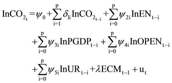 (12)
(12)
where ECMt–1 is the error correction term which is obtained from the following estimated cointegration equation
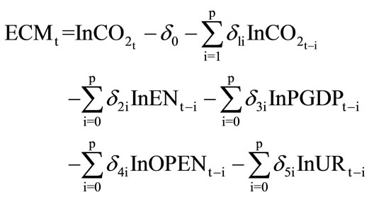 (13)
(13)
In this case the parameter λ represents the speed of adjustment for short-run to reach in the long-run equilibrium. The long-run and also the short-run elasticities of CO2 with respect to EN, PGDP, OPEN and UR are given below in Tables 5 and 6.
From estimated results in Table 5 it has been found that for a 100% increase in energy consumption leads to increase 109.7% in carbon dioxide emissions in long-run which is statistically significant at any significance level. The elasticity of carbon dioxide emissions with respect to trade openness is −0.1306, suggesting that for increasing 100% foreign trade the carbon dioxide emissions is decreasing 13.06% and the contribution of foreign trade in Japan statistically significant at 10% level of significance. But in case of per capita GDP (PGDP), and urbanization (UR), the relationships are insignificant with carbon dioxide emissions. The error correction mechanism (ECM) is employed to check the short-run relationship among
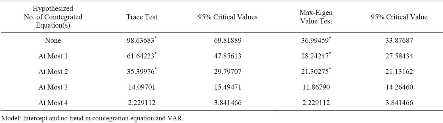
Table 4. Results of the Johansen and Juseliues’s cointegration test.
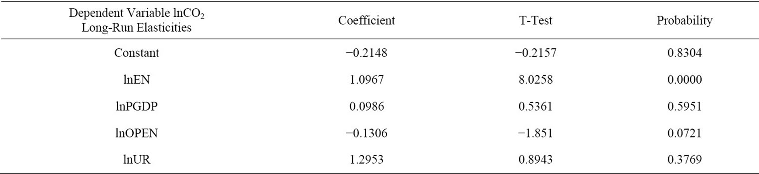
Table 5. ARDL coefficients for long-run.
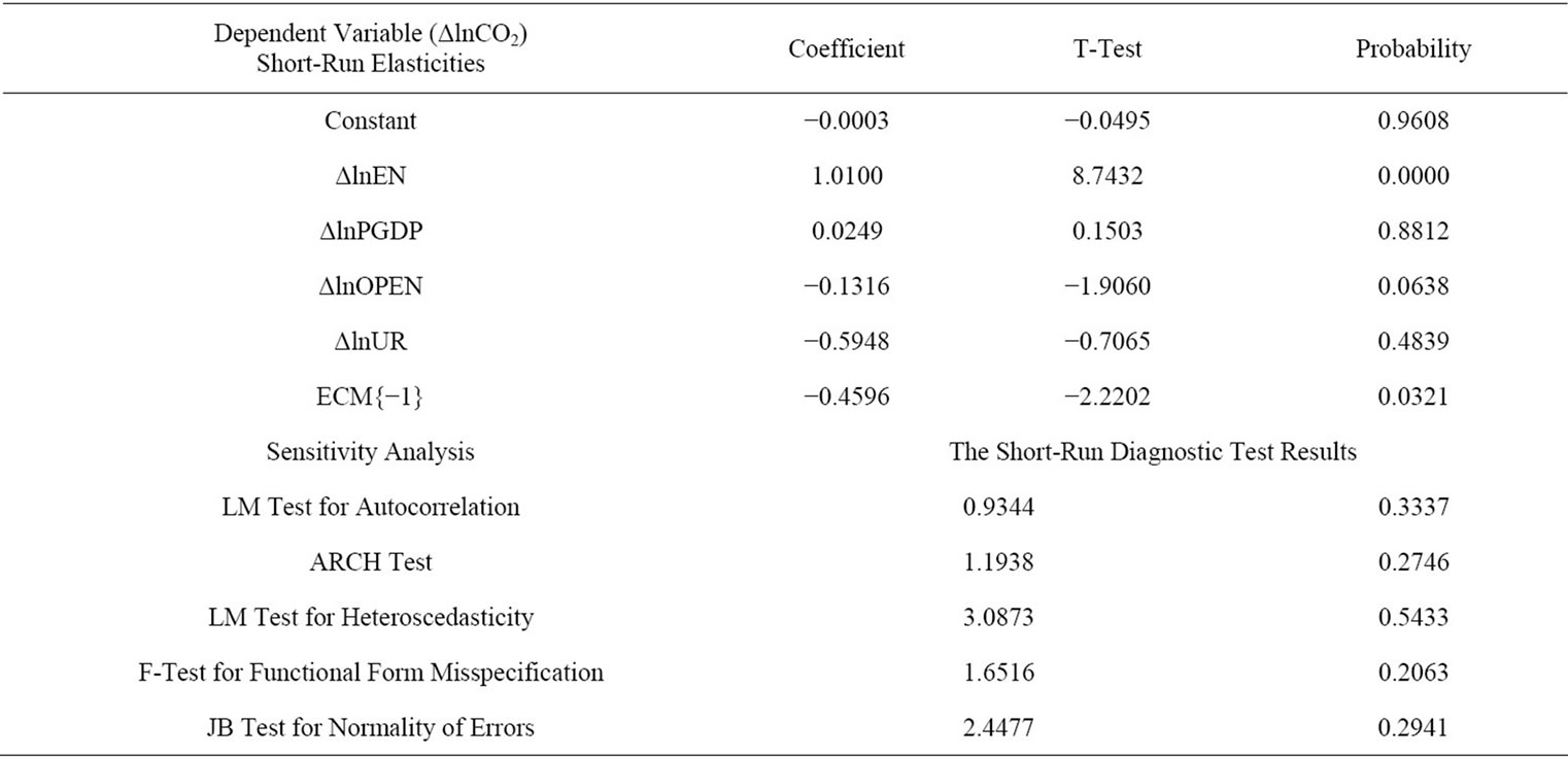
Table 6. Error correction model for short-run elasticity.
the variables.
The Table 6 shows that the coefficient of ECM (−1) is statistically significant at 5% level of significance which indicates that speed of adjustment for short-run to research in the long-run equilibrium is significant. The error correction term is statistically significant and it’s magnitude is quite higher indicates a faster return to equilibrium in the case of disequilibrium. The error correction term is −0.46 with the expected sign, suggesting that when per capita carbon dioxide emissions is above or below its equilibrium level, it adjusts by almost 46% within the first year. The full convergence process to its equilibrium level takes about more than two years. Thus the speed of adjustment is significantly faster in the case of any shock to the carbon dioxide emissions equation. The environmental quality is not found to be good in respect of energy consumption in Japan, because the long-run elasticity of CO2 emissions with respect to energy consumption (1.0967) is higher than short run elasticity of 1.01. This means that over time higher energy consumption in Japan gives rise to more CO2 emissions and the environment will be polluted more. But in respect of other variables economic growth, trade openness and urbanization the environmental quality is found to be normal good in the long-run.
Sensitivity analysis: Diagnostic tests for serial correlation, autoregressive conditional heteroscedasticity, heteroscedasticity, functional form misspecification and non-normal errors are conducted and the results are reported in Table 6. The test results indicate that there is no evidence of serial correlation, because the functional form is well specified and there is no problem of heteroscedasticity. Also the autoregressive conditional heteroscedasticity is not present in the short-run model. The test results also support that there is no problem of normality of random error terms in Equation (12).
5.3. Granger Causality Test
The cointegration relationship indicates the existence of causal relationship between variables but it does not indicate the direction of causal relationship between variables. Therefore it is common to test for detecting the causal relationship between variables using the Engle and Granger [51] test procedure. There are three different models that can be used to detect the direction of causality between two variables X and Y depending upon the order of integration and the presence or absence of cointegration relationship. If two variables say X and Y are individually integrated of order one I(1) and cointegrated, then Granger causality test may use I(1) data because of super consistency properties of estimators. If X and Y are I(1) and cointegrated, the Granger causality test can be applied to I(0) data with an error correction term. If X and Y are I(1) but not cointegrated, Granger causality test requires transformation of the data to make I(0).
For this paper, the presence of cointegration relationship the application of Engle and Granger (1987) causality test in the first differenced variables by means of a VAR will misleading the results, therefore an inclusion of an additional variable to the VAR system such as the error correction term would help us to capture the longrun relationship. The augmented form of the Granger causality test involving the error correction term is formulated in a multivariate pth order vector error correction model given as below;
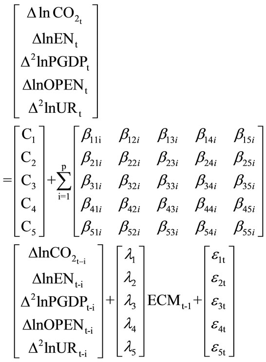 (14)
(14)
where, t = p + 1, p + 3,···, T; The C’s, β’s and λ’s are the parameters to be estimated. ECMt–1 represents the one period lagged error-term derived from the cointegration vector and the ε’s are serially independent with mean zero and finite covariance matrix. From the Equation (14) given the use of a VAR structure, all variables are treated as endogenous variables. The F test is applied here to examine the direction of any causal relationship between the variables. The energy does not Granger cause CO2 emissions in the short run, if and only if all the coefficients β12i’s  are not significantly different from zero in Equation (14). Similarly the CO2 emissions do not Granger cause energy in the short run if and only if all the coefficients β21i’s
  are not significantly different from zero in the Equation (14). There are referred to as the short-run Granger causality test. The coefficients on the ECM represent how fast deviations from the long-run equilibrium are eliminated. Another channel of causality can be studied by testing the significance of ECM’s. This test is referred to as the long run causality test. The panel short-run and long-run Granger causality results are reported below in Table 7.
The reported values in parentheses are the p-values of the test. The findings in Table 7 indicates that short-run unidirectional causality running from energy consumption and trade openness to carbon dioxide emissions, from trade openness to energy consumption, from carbon dioxide emissions to economic growth, and from economic growth to trade openness in Japan. It has been found that the error correction terms are statistically significant which indicate that there exist a long-run relationship among the variables in the form of Equation (1) which also conform the results of bounds test and Johansen
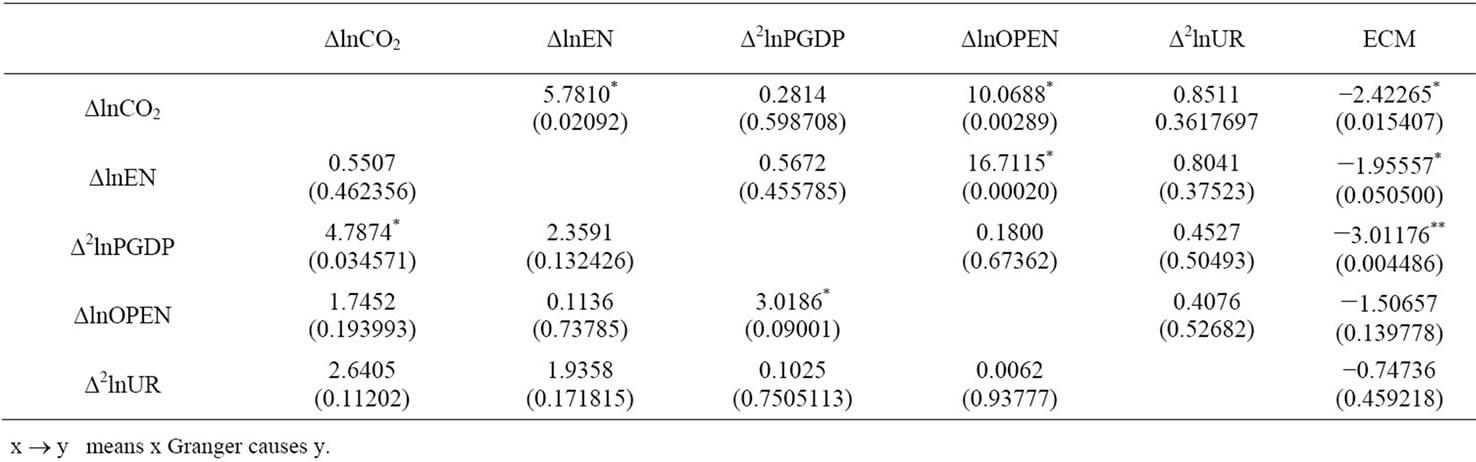
Table 7. Granger F-test results.
and Juseliues’s [50] conintegration test.
5.4. CUSUM and CUSUMSQ Tests
Finally the stability of the long-run parameters together with the short-run movements for the equations has been examined using cumulative sum (CUSUM) and cumulative sum of squares (CUSUMSQ) tests proposed. The related graphs of these tests are presented below in Fig ures 2 and 3. From Figures 2 and 3 it can be seen that the CUSUM and CUSUMSQ tests results are within the critical bounds implying that all coefficients in the error correction model are stable. Therefore the preferred CO2 emissions model can be used for policy decision making purpose, such that the impact of policy changes considering the explanatory variables of CO2 emissions equation will not cause major distortion in the level of CO2 emissions, since the parameters in this equation seem to follow a stable pattern during the estimation period.
6. Conclusions and Policy Implications
This paper attempts to investigate empirically the dynamic causal relationships between CO2 emissions and energy consumption, economic growth, foreign trade and urbanization of Japan through the cointegration and causality analysis. The bounds testing approach is applied for cointegration in order to examine the existence of long-run equilibrium relationship between CO2 emissions and its determinants, also the Johansen and Juseliues’s conintegration test is applied in order to find the existence of cointegration equations as the robustness of bounds test. Furthermore, the Granger causality test is applied with VEC model to investigate the causal linkage between different pairs of variables.
Firstly, it is found that CO2 emissions, energy consumption, economic growth, foreign trade and urbanization are cointegrated. This implies that the explanatory variables energy consumption, economic growth, foreign trade and urbanization are coalescing with CO2 emission
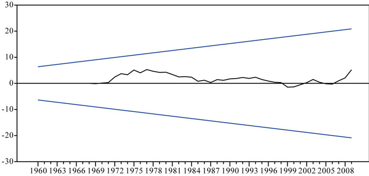
Figure 2. Plot of cumulative sum of recursive residuals. The straight lines represent critical bounds at 5% significance level.
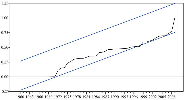
Figure 3. Plot of cumulative sum of squares of recursive residuals. The straight lines represent critical bounds at 5% significance level.
to achieve their steady-state equilibrium in the long-run, although deviations may occur in the short-run. From the bounds tests and Johansen and Juseliues’s, it is found that there are at least three cointegration equations among these variables. It is found that the long-run elasticity of CO2 emissions with respect to energy consumption (1.097) is higher than short run elasticity of 1.01. This indicates that the environmental quality is not found to be good in respect of energy consumption in Japan. This means that over time higher energy consumption in Japan gives rise to more CO2 emissions as a result the environment will be polluted more. The variable economic growth and urbanization has positive impact and trade openness has negative impact on CO2 emissions in the long-run but not statistically significant at all. Thus in respect of economic growth, trade openness and urbanization the environmental quality is found to be normal good in the long-run in Japan.
The Granger causality test results support the existence of unidirectional short-run causal relationship from energy consumption and trade openness to CO2 emissions, from trade openness to energy consumption, from CO2 emissions to economic growth, and economic growth to trade openness. It is found that the error correction terms in VEC model are statistically significant when CO2 emissions, energy consumption and economic growth are individually dependent variable. This indicates that there exists a long-run relationship among the variables in the form of Equation (1).
The CUSUM and CUSUMSQ tests results suggest the policy changes considering the explanatory variables of CO2 emissions equation will not cause major distortion in the level of CO2 emissions.
Since a unidirectional causality from CO2 emissions to economic growth in Japan is found thus any policy in respect of reduction of CO2 emissions will be harmful for further economic development in Japan. The reduction of CO2 emissions could lead to fall in economic growth in Japan as a result the unemployment rate will increase in future which is already running at around 4.6% in Japan.
It is found that the long-run as well as short-run energy consumption has significant positive impact on carbon dioxide emissions, implies that due to expansion of the industrial output for economic development of Japan are consuming more energy, which pressure on the environment leading to more emissions, thus it is very essential to apply some sort of pollution control action in Japan with respect of energy consumption.
From the analytical results the following points may be suggested to implement to control CO2 emissions. Japan need to embrace more energy conservation policies in order to reduce carbon dioxide emissions and they should consider strict environmental and energy policies. The research and investment in clean energy should be an integral part of the process of controlling the carbon dioxide emissions and have to find the alternative sources of energy to oil and to sustainable economic growth. Thus implementing the environmental and energy policies and also reconsidering the strict energy policies Japan can control CO2 emissions.
REFERENCES
- P. K. Narayan and S. Narayan, “Carbon Dioxide and Economic Growth: Panel Data Evidence from Developing Countries,” Energy Policy, Vol. 38, No. 1, 2010, pp. 661- 666.
- U. Soytas and R. Sari, “Energy Consumption and GDP: Causality Relationship in G-7 Countries and Emerging Markets,” Energy Economics, Vol. 25, No. 1, 2003, pp. 33-37.
- G. M. Grossman and A. B. Krueger, “Environmental Impacts of the North American Free Trade,” 1991. http://www.nber.org/papers/w3914.pdf.
- N. Shafik, “Economic Development and Environmental Quality: An Econometric Analysis,” Oxford Economic Papers, Vol. 46, 1994, pp. 757-773.
- S. Dinda and D. Coondoo, “Income and Emissions: A Panel Based Cointegration Analysis,” Ecological Economics, Vol. 57, No. 2, 2006, pp. 167-181.
- M. T. Heil and T. M. Selden, “Carbon Emissions and Economic Development: Future Trajectories Based on Historical Experience,” Environmental and Development Economic, Vol. 6, No. 1, 2001, pp. 63-83.
- B. Friedl and M. Getzner, “Determinants of Co2 Emissions in a Small Open Economy,” Ecological Economics, Vol. 45, No. 1, 2003, pp. 133-148.
- J. Kraft and A. Kraft, “On the Relationship between Energy and GNP,” Journal of Energy and Development, Vol. 3, No. 2, 1978, pp. 401-403.
- A. M. N. Masih and R. Masih, “Energy Consumption, Real Income and Temporal Causality: Results from Multi-Country Study Based on Cointegration and Error-Correction Modeling Techniques,” Energy Economics, Vol. 18, No. 3, 1996, pp. 165-183.
- H. Y. Yang, “A Note on the Causal Relationship between Energy and GDP in Taiwan,” Energy Economics, Vol. 22, No. 3, 2000, pp. 309-317. doi:10.1016/S0140-9883(99)00044-4
- Y. Wolde-Rufael, “Energy Consumption and Economic Growth: The African Experience Revisited,” Energy Economic, Vol. 31, No. 2, 2009, pp. 217-224.
- P. K. Narayan and B. Singh, “The Electricity Consumption and GDP Nexus for the Fiji Islands,” Energy Economics, Vol. 29, No. 6, 2007, pp. 1141-1150.
- P. K. Narayan and S. Russell, “Energy Consumption and Real GDP in G7 Countries: New Evidence from Panel Cointegration with Structural Breaks,” Energy Economics, Vol. 30, No. 5, 2008, pp. 2331-2341.
- J. B. Ang, “Are Saving and Investment Cointegrated? The Case of Malaysia (1965-2003),” Applied Economics, Vol. 39, No. 17, 2007, pp. 2167-2174.
- U. Soytas, R. Sari and B. T. Ewing, “Energy Consumption, Income, and Carbon Emissions in the United States,” Ecological Economics, Vol. 62, No. 3, 2007, pp. 482-489.
- F. Halicioglu, “An Econometric Study of CO2 Emissions, Energy Consumption, Income and Foreign Trade in Turkey,” Energy Policy, Vol. 37, No. 3, 2009, pp. 1156- 1164.
- A. Tamazian and B. B. Rao, “Do Economic, Financial and Institutional Developments Matter for Environmental Degration? Evidence from Transitional Economies,” Energy Economics, Vol. 32, No. 2, 2010, pp. 137-145.
- H. H. Lean and R. Smyth, “Co2 Emissions, Electricity Consumption and Output in ASEAN,” Applied Energy, Vol. 87, No. 6, 2010, pp. 1858-1864.
- E. Akbostaci, S. Turut-Asik and G. Tunc, “The Relationship between Income and Environment in Turkey: Is There an Environmental Kuznets Curve?” Energy Policy, Vol. 37, No. 3, 2009, pp. 861-867.
- A. T. Akarca and I. T. B. Long, “On the Relationship between Energy and GNP: A Reexamination,” Journal of Energy and Development, Vol. 5, No. 2, 1980, pp. 326- 331.
- E. S. H. Yu and B. K. Hwang, “The Relationship between Energy and GNP: Further Results,” Energy Economics, Vol. 6, No. 3, 1984, pp. 186-190. doi:10.1016/0140-9883(84)90015-X
- D. I. Stern, “Energy Growth in the USA: A Multivariate Approach,” Energy Economics, Vol. 15, No. 2, 1993, pp. 137-150.
- B. S. Cheng, “An Investigation of Cointegration and Causality between Energy Consumption and Economic Growth,” Journal of Energy and Development, Vol. 21, No. 1, 1995, pp. 73-84.
- E. S. H. Yu and J. Y. Choi, “The Causal Relationship between Energy and GNP: An International Comparison,” Journal of Energy and Development, Vol. 10, No. 2, 1985, pp. 249-272.
- U. Erol and E. S. H. Yu, “On the Causal Relationship between Energy and Income for Industrialized Countries,” Journal of Energy and Development, Vol. 13, No. 1, 1987, pp. 113-122.
- A. M. N. Masih and R. Masih, “On the Temporal Causal Relationship between Energy Consumption, Real Income, and Prices: Some New Evidence from Asian-Energy Dependent NICs Based on a Multivariate Cointegration/ Vector Error-Correction Approach,” Journal of Policy Modeling, Vol. 19, No. 4, 1997, pp. 417-440. doi:10.1016/S0161-8938(96)00063-4
- Y. U. Glasure, “Energy and National Income in Korea: Further Evidence on the Role of Omitted Variables,” Energy Economics, Vol. 24, No. 4, 2002, pp. 355-365.
- W. Oh and K. Lee, “Causal Relationship between Energy Consumption and GDP Revisited: The Case of Korea 1970-1999,” Energy Economic, Vol. 26, No. 1, 2004, pp. 51-59.
- J. Asafu and Adjaye, “The Relationship between Energy Consumption, Energy Prices and Economic Growth: Time Series Evidence from Asian Developing Countries,” Energy Economics, Vol. 22, No. 6, 2000, pp. 615-625.
- P. K. Narayan and R. Smyth, “Energy Consumption and Real GDP in G7 Countries: New Evidence from Panel Cointegration with Structural Breaks,” Energy Economics, Vol. 30, No. 5, 2008, pp. 2331-2341. doi:10.1016/S0140-9883(00)00050-5
- B. S. Cheng, “Causality between Energy Consumption and Economic Growth in India: An Application of Cointegration and Error Correction Modeling,” Indian Economic Review, Vol. 34, No. 1, 1999, pp. 39-49.
- Y. Chang and J. F. Wong, “Poverty, Energy, and Economic Growth in Singapore,” Working Paper 37, Department of Economics, National University of Singapore, 2001,
- Y. U. Glasure and A. R. Lee, “Cointegration, Error Correction and the Relationship between GDP and Energy: The Case of South Korea and Singapore,” Resource and Energy Economics, Vol. 20, No. 1, 1998, pp. 17-25. doi:10.1016/S0928-7655(96)00016-4
- U. Soytas and R. Sari, “Energy Consumption and GDP: Causality Relationship in G-7 Countries and Emerging Markets,” Energy Economics, Vol. 25, No. 1, 2003, pp. 33-37.
- B. S. Cheng and T. W. Lai, “An Investigation of Cointegration and Causality between Energy Consumption and Economic Activity in Taiwan,” Energy Economics, Vol. 19, No. 4, 1997, pp. 435-444. doi:10.1016/S0140-9883(97)01023-2
- G. M. Grossman and A. B. Krueger, “Environmental Impacts of the North American Free Trade,” 1991. http://www.nber.org/papers/w3914.pdf.
- R. Andersson, J. M. Quigley and M. Wilhelmsson, “Urbanization, Productivity, and Innovation: Evidence from Investment in Higher Education,” Journal of Urban Studies, Vol. 66, No. 1, 2009, pp. 2-15.
- H. Y. Toda and T. Yamamoto, “Statistical Inference in Vector Autoregression with Possibly Integrated Processes,” Journal of Econometrics, Vol. 66, No. 1-2, 1995, pp. 225-250.
- U. Soytas and R. Sari, “Energy Consumption, Economic Growth, and Carbon Emissions: Challenges Faced by an EU Candidate Member,” Ecological Economics, Vol. 68, No. 6, 2009, pp. 1667-1675.
- X.-P. Zhang and X.-M. Cheng, “Energy Consumption, Carbon Emissions, and Economic Growth in China,” Ecological Economics, Vol. 68, No. 10, 2009, pp. 2706- 2712.
- R. Sari and U. Soytas, “Are Global Warming and Economic Growth Compatible? Evidence from Five OPEC Countries,” Applied Energy, Vol. 86, No. 10, 2009, pp. 1887-1893.
- A. Jalil and S. F. Mahmud, “Environment Kuznets Curve for CO2 Emissions: A Cointegration Analysis for China,” Energy Policy, Vol. 37, No. 12, 2009, pp. 5167-5172.
- J. H. Stock and M. W. Watsos, “Testing for Common Trends,” Journal of the American Statistical Association, Vol. 83, No. 403, 1988, pp. 1097-1107.
- C. W. J. Granger and P. Newbold, “Spurious Regression in Econometrics,” Journal of Econometrics, Vol. 2, No. 2, 1974, pp. 111-120.
- P. C. B. Phillips, “Understanding Spurious Regression in Econometrics,” Journal of Econometrics, Vol. 33, No. 3, 1986, pp. 311-340.
- D. A. Dickey and W. A. Fuller, “Distribution of the Estimators for the Autoregressive Time Series with a Unit Root,” Journal of the American Statistical Association, Vol. 79, No. 386, 1979, pp. 355-367.
- P. C. B. Phillips and P. Perron, “Testing for a Unit Root in Time Series Regression,” Biometrika, Vol. 75, No. 2, 1987, pp. 335-346.
- J. MacKinnon, “Critical Values for Cointegration Tests,” In: R. F. Engle and C. W. J. Granger, Eds., Long-Run Economic Relationship, Reading in Cointegration, Oxford University Press, Oxford, 1990
- M. H. Pesaran, Y. Shin and R. J. Smith, “Bound Testing Approaches to the Analysis of Level Relationships,” Journal of Applied Econometrics, Vol. 16, No. 3, 2001, pp. 289-326.
- S. Johansen and K. Juselius, “Maximum Likelihood Estimation and Inference on Cointegration-with Application to the Demand for Money,” Oxford Bulletin of Economics and Statistics, Vol. 52, No. 2, 1990, pp. 169- 210.
- R. Engle and C. Granger, “Cointegration and Error Correction Representation: Estimation and Testing,” Econometrica, Vol. 55, No. 2, 1987, pp. 251-276.
NOTES
1Total GHG (Kyoto gases) emissions in 2004 amounted to 49.0 GtCO2- eq, which is up from 28.7 GtCO2-eq in 1970—a 70% increase between 1970 and 2004. In 1990 global GHG emissions were 39.4 GtCO2-eq.
2Some of the studies include those for China (Shiu and Lam 2004), Fiji (Narayan and Singh 2007), India (Masih and Masih 1996), Indonesia (Asafu-Adjaye 2000), Philippines (Yu and Choi 1985), Sri Lanka (Moritomo and Hope 2004), Taiwan (Yang 2000), Turkey (Soytas and Sari 2003, Altinay and Karagol 2005), and Venezuela (Squalli 2007).