Open Journal of Modelling and Simulation
Vol.02 No.04(2014), Article ID:50997,9 pages
10.4236/ojmsi.2014.24016
Partial Availability and RGBI methods to improve system performance in different interval of time: The Drill Facility System Case study
Eduardo Calixto1, Gilson Brito de Lima Alves Gilson2, Adelci Menezes de Oliveira3
1UFRJ-COPPE, Rio de Janeiro, Brazil
2UFF-LATEC, Rio de Janeiro, Brazil
3Petrobras S.A., Rio Grande do Norte, Brazil
Email: eduardo.calixto@hotmail.com
Copyright © 2014 by authors and Scientific Research Publishing Inc.
This work is licensed under the Creative Commons Attribution International License (CC BY).
http://creativecommons.org/licenses/by/4.0/


Received 29 July 2014; revised 30 August 2014; accepted 25 September 2014
ABSTRACT
The main objective of this study is to propose a methodology to define the operational availability for a system in different interval of time based on Monte Carlo simulation. In addition, it is also an objective to identify critical equipment in such interval of time and define when carrying out inspections to detect and prevent failures. Nowadays, many software packages which apply Monte Carlo simulation based on reliability diagram block do not show the operational availability defined by interval of time. In most of cases, there’s no result that shows how system performs in specific interval of time. Depending on situation, it’s important to define the operational availability by different interval of time in order to follow up system performance along time. In order to solve such problem, it is proposed the “partial availability methodology” based on system age. Indeed, such method regards equipment age based in different period of time that will results in Partial Availability. That means, as instance, in case of two years of simulation there will be the cumulative operational availability and partial operational availability results for first and second years for example. Therefore, it is also important to define the inspection time in each interval of time (year) in order to detect possible equipment failure and define preventive maintenance to avoid such failures that will be performed by RGBI method. In order to show such methodologies, it will be carried out a drill facility case study which is required to define operational availability of the system on the first and second years as well as inspection time.
Keywords:
Partial Operational Availability, System Age, Probability Density Function (PDF), Reliability Growth Based Inspection (RGBI)

1. Introduction
Nowadays, different types of software applied on RAM analysis are based on Monte Carlo Simulation method and the final result is the cumulative operational availability. Indeed, such result is cumulative along simulation time; in another words, it takes into account all system downtime along simulation period of time to calculate the operational availability [1] . Whenever a high performance system is in context, such result will be accomplished as expected, because the defined period of simulation is appropriated to operational availability target. By the other way round, it’s not possible to verify the operational availability in a specific interval of time.
Actually, for system with high operational availability performance, the partial result is not a problem because when such system achieves operational availability target in cumulative period of time, they mostly achieve availability target in specific interval of times as well. Even though, it is necessary in some cases to find out the operational availability in different intervals of time to follow up system performance or even establish operational availability targets for different interval of time.
In some cases, in order to plan resources like component stock, services order as well as plan preventive maintenance, it is very important to know which operational availability system will achieve in specific interval of time. Therefore, such partial operational availability result is important to find out which equipment will fail in such interval of time. Indeed, that is usual for system that achieves low operational availability when considering long cumulative period of time. Therefore, in these cases, operational availability is defined for the short period of time. Nevertheless, most of software does not take into account the operational availability in different interval of time because the simulation result shows only the cumulative operational availability along years.
Once we face such situation, a possible solution is to define a fixed period of time like one year as instance and simulate the system life cycle year by year. It means that all simulations will be performed for one calendar year but will consider the system age. By this way, on second year for example the system is one year older and the simulation will describe what happen during the second year.
In addition, more than define the partial operational availability, it’s also important to define the critical equipment, the best inspection and preventive maintenance time in order to avoid failures.
Unfortunately, in many cases the operational availability is defined for a specific interval of time by calculating the average of cumulative operational availability per time. Indeed, that will not solve the problem because it is also important to verify which equipment fails in different interval of time in order to prevent such failures.
The proposal paper will present “the partial availability” and “RGBI” methodologies applying a drill facilities case study in order to improve such system performance.
2. partial Availability
The Monte Carlos simulation in RAM analysis has the main objective to define system operational availability and critical equipments in order to support decisions by implementing improvements actions when it’s necessary [2] . Such operational availability result is cumulative along simulation time and to have partial operational availability values two approaches are possible.
Þ Discounting time on PDF (Probability Density Function) parameters.
Þ Accounting age on simulation time.
On first case, to regards change in PDF parameters is necessary to discount time on position parameter in order to not modify PDF characteristic so if intended for example to anticipate in equipment age in one year, such value is discounted in position parameter and if necessary to postpone one year is add such value in position parameter. That’s easy to realize if it been considering a PDF with Gaussian shape like normal, lognormal, gumbel, logistic and loglogistic. figure 1 shows normal PDF with position parameter discounted in one year in order to simulate the second year of such equipment life and find out operational availability on this interval of time. The blue PDF in figure 1 is original PDF and the black one is the time discounted PDF. The equipment Operational availability is 100% in one year because there’s no failure (normal PDF: m = 2, s = 0.1). In addition, to find out the equipment operational availability on second operational year is discounted one year in position parameter (m = 2 − 1 ® m = 1). Thus, the Monte Carlo simulation is carried out regard one year of simulation time.

Figure 1. PDF parameters discounted time.
Actually, when position parameter is discounted in one year, whether further interval of time is simulated the failure will occur earlier than expected. Thereby, such approach is correct only when the position parameter discounted by specific time is higher or equal than period of simulation time.
In case of others PDF with no Gaussian characteristics such limitation is similar. Whether such approach is applied to a general PDF like Weilbul 3P for example, is necessary to discount time to location parameter. As instance, if the location parameter value is five years and is intended to know about the second year, so once the location parameter is discounted in one year the next step is perform simulation for one year.
Indeed, the limitation in such approach is that such simulation results works only for the first failure. The following failure will occur earlier than simulation result because the real PDF parameter is discounted.
In Weibul 3P case for example, once the location parameter (g) is discounted, the second failure will earlier than expected. For example if is intended to simulate fifth year and the location parameter value is five, once the location parameters (g) is discounted the first failure occur in one year of simulation as expected but the second one would also happen previously because the position parameter was discounted. Thereby, under such circumstance, the location or position parameter must be updated constantly to reproduce the partial availability for the wanted interval of time.
In addition, if it being considered that after repairs, equipments is as good as new, such earlier failure can not happen. In case of as bad as old, is acceptable that failure occurs in short period of time after repair but that is not expected [3] . figure 2 shows an example of Monte Carlo simulation to describe draw work failure behavior on second operational year regards one year discounted in PDF location parameter (g). The draw work failure is represented by the Weibull 3P PDF which parameters are b = 2.01, h = 0.29, g = 0.86. Regarding that the location parameter (g = 0.86) is discounted in one year in order to simulate the second year, the new PDF parameters will be (b = 2.01, h = 0.29, g = 0). Therefore, when location parameter is discounted and such value is not less than simulation period of time, the second failure will not take into account on the period of time of 0.86 years as shown figure 2. Thus the MTBF is 3625 when would be 7533 h (g = 0.86).
In order to avoid such problem, the second possibility is to take into account system age to find out partial operational availability in different interval of time that regards only downtimes occurred in such interval of time.
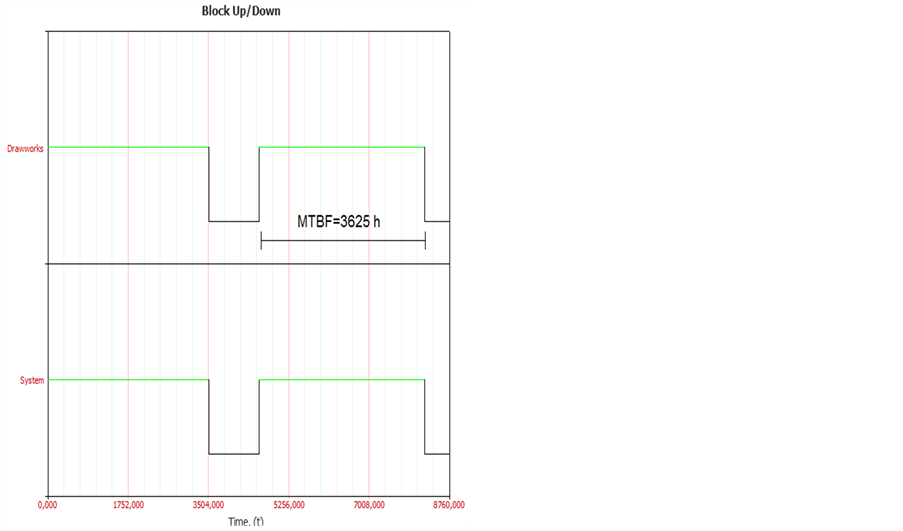
Figure 2. Drawwork (second year simulated).
The operational availability most be defined as total time which system is available to operate (uptime) by total nominal time as shows equation below.

where:
 = real time when system is available;
 = nominal time when system must be available.
As mentioned before, mostly, the Monte Carlo simulation shows cumulative operational availability but to know partial operational availability in different interval of times it is necessary to define such periods of times along total period of time and then account downtimes in each period of time. figure 3 shows an example of time line T (0, n) divided in three interval of time.
The equation which represents Operational availability along T (0, n) is:

Indeed, regarding three different interval of times, the operational availability along each period of time will be:
Period I

Period II

Figure 3. Time line T (0, n).

Period III

where:
 = real time when system is available;
 = nominal time when system must be available.
It is possible to considers as many interval time as necessary depends on requirements and available data. In this specific case, when Monte Carlo simulation is performed, it is necessary to define start age for system and regards one year as simulation period of time. Thus, age for first year is zero, for second is one and for third is two years.
Once system age is considered in Monte Carlos simulation, the simulation results shows always what happen after aged time that is the interval of time that must be defined the operational availability and critical equipment.
Despite a correct approach, whenever is required to know about one specific period of time it will be necessary to age all equipment represented on RBD (reliability block diagram) or FTA (fault tree analysis).
Such approach would be included in software packages to show the results in different interval of time automatically.
3. reliability Growth Based Inspection (RGBI)
Indeed, it is not always possible to overhaul the critical equipment defined by Monte Carlo simulation by partial Availability methodology. In this case, it is necessary to define inspection time to check equipment condition in order to define preventive maintenance time in order to avoid equipment failures.
In this section is proposed the reliability growth method (Crow AMSAA) to predict the inspection time for different interval of time.
The reliability growth approach is applied to product development and support decisions to achieve reliability targets after improvement have been implemented [4] .
Various mathematical equations models may be applied in reliability growth analysis depend on how the test is carried out as well as the type of data. Such methods are:
· Duanne;
· Crow Ansaa;
· Crow Extended;
· Lloyd Lipow;
· Gompertz;
· Logistic;
· Crow Extended; and
· Gompertz.
The reliability growth based inspection (RGBI) method will regards Crown AMSAA analysis methodology to estimate future inspections that is also applied to assess reparable systems (equipment). Thus, regarding complete data which include repairs, the Non-Homogeneous Poisson Process is applied [5] , as shown in equation (1) below:
Equation (1)

The expected cumulative number of failure can be described also by equation (2) below:
Equation (2)

To determine the inspection time, it is necessary to use the cumulative number of failure function and, based on equipment failure data, to define the following cumulative failure number. Based on this number, it is necessary to reduce from such time the required time to carry out inspection task regarding the P-F interval (potential and functional failure time).
In fact, applying such methodology for drilling diesel motor is possible to predict when the next failure time will occur and if reducing this time by time required to perform inspection we have the start inspection time. The cumulative number of failures is ten. Therefore, applying the expected cumulative number of failures and using the Crown AMSAA function parameters (l = 1.15 and b = 1.02) in equation (1), the next failure will expected to occur in 8.32 years as shown in equation (3).
Equation (3)

The next item will apply a case study concerning the both methods in order to show the advantages to define system performance in different interval of time as well as inspection time to keep such performance.
4. Drill Facilities Case Study
4.1. Partial Availability Case Study
In order to clarify partial availability approach, such method will be applied in drill facility case study which system availability target is 90% annually. In addition, it is necessary to define stock policy and maintenance policy for two years based in RAM analysis results.
Indeed, the drill facility do not achieve high performance for over one year and some equipment failures happen on first year and others on second year. Therefore, will be carried out two simulation regarding equipments age in order to define availability and critical equipments for first and second year. Before modeling RDB (reliability diagram block) was performing equipment lifetime data analysis and one of the most critical equipment is the compressor from air compressor subsystem. table 1 shows an example of compressor failure PDF.

Table 1. Failure data.
After carry out the lifetime data analysis, the RBD was build up regarding the six subsystem which drill facility system comprises as shows figure 4.
Performing simulation for the first year, system achieve 85.44% of operational availability in one year and is expected 23 failures.
The operational availability rank is an important index to support improvement decision [6] . Indeed, once equipment in each subsystem are mostly in series. By this way, compressor is the availability bottle neck because have the lowest availability of drill facility system. The availability rank is shown in table 2.
Once the compressor is the most critical equipments, as recommendation was proposed to analyze the others compressor reliability and compare among than which is the highest reliability in order to define higher reliability requirement for compressors suppliers companies. Indeed it is expected to compressor achieve at least 100% of reliability in two year. Unfortunately, in drill facility system the compressor achieves 88.58% of availability in one year. Consequently, some improvement is required in compressor.
Therefore, the following action is to define better reliability requirements for diesel pump or install other stand by pump to achieve 100% of availability in at least one year as required.
Regarding this additional recommendation, the drill facility system will achieve 91.87% in one year, being a little higher than the initial operational availability target that was 90% in one year.
Applying the partial availability methods to analyze the second year, the drill facility system availability in second year is 68.84% if no improvement in compressor be carried out. Even though, regarding high compressor reliability, that means implement improvement action on the first year, the drill facility system will achieve 81.95% on second year. Actually, on second year other equipments take place as more critical in terms of impact in system operational availability. table 3 shows availability rank on second operational year.
Despite improvement in compressor, some other improvement in Transmission Box is required to enable the system achieve operational availability target (90% in one year). Therefore, reliability requirements must be defined for such equipment. Indeed, wear out is usual in such equipment and even if it’s possible to have 100% of reliability for such equipment, it is advisable to perform inspections and preventive maintenance whenever it’s possible in order to keep transmission box available as long as possible on second year.
Thereby, if transmission box achieve 100% of operational availability on second year, drill facility system will achieve 91.25 % of operational availability on second year.
4.2. Reliability Growth Based Inspection (RGBI) case study
In order to define the critical equipment inspection time, it is necessary to use the cumulative number of failure function and, based on equipment failure data, to define the following cumulative failure number. Based on this number, it is necessary to reduce from such time the required time to carry out inspection task regarding the P-F interval (potential and functional failure time).
In fact, applying such methodology for drilling diesel motor is possible to predict when the next failure time will occur and if reducing this time by time required to perform inspection we have the start inspection time. The cumulative number of failures is ten. Therefore, applying the expected cumulative number of failures and using the Crown AMSAA function parameters (l = 1.15 and b = 1.02) in equation (1), the next failure will expected to occur in 8.32 years as shown in Equation (1) as described above.
Equation (1)

Figure 4. Drill facility subsystems.
Table 2. Availability rank (year I).
Table 3. Availability rank (year II).

The same approach is used to define the following failure using equation (2), in which eleven is used as the expected cumulative number of failures as shown in equation (2).
Equation (2)

In equation (3) below, the expected number of failures used is twelve.
Equation (3)

After defining the expected time of the next failure, it is possible to define the appropriate inspections period of time. Whether is being considered one month (0.083 year) as an adequate time to start each inspection the following inspection time after ninth, tenth and eleventh failure are:
Þ1˚ Inspection—8.23 year (8.32 − 0.083);
Þ2˚ Inspection—9.07 year (9.15 − 0.083);
Þ3˚ Inspection—9.87 year (8.32 − 0.083);
The remarkable point is that such methodology regards reliability growth or degrades to predict the following failures along time. In RGBI method, whenever new failures occur, it is possible to update the model and get more accurate values of cumulative expected number of failure.
The example of cumulative failure plotted against time for a diesel motor is presented in figure 5, using cumulative failure function parameters b = 1.02 and l = 1.15. Based on such analysis, is possible to graphically observe that the next failures (failures 10˚, 11˚ and 12˚) will occur on 8.32; 9.15 and 9.96 years, respectively. That means 0.92; 1.75 and 2.56 year after last failure (7.4 years).
Despite simple application, RGBI analysis requires first to have Crown AMSAA parameters model to have cumulative expected number of failure. Such parameters can be estimate by Maxi likelihood method by using software application. In doing so, whenever it is possible, is advisable to use software to plot directly the expected number of failures graphs. In this case, is possible to update historical data with new data and plot expected future failures directly on graph.
Applying such methodology for other drill facility equipments is possible to define inspection period of time and depend o inspection results preventive maintenance may be plan to anticipate equipment fail.
Table 4 shows inspection policy defined for Compressor, Diesel Motor, Crown Block and Transmission

Figure 5. Inspection Based in reliability growth.
Table 4. Inspection based in reliability growth.
Box. Actually, despite Inspection Based in Growth reliability define an exactly time to inspection, addition information is must to be considered like logistic time to perform inspection. Indeed, such time must be discounted of inspection time in order to define a range of time to carry out inspection in each equipment. In Drill Facility System equipments was defined one month (0.083) to perform inspection and such time is discounted by expected failure time. Once again it is important to be aware about the P-F interval of time.
5. Conclusions
The partial availability methodology has demonstrated how to perform RAM analysis considering different interval of time for system which has no high performance for long period of time. Therefore, it’s possible to assess such system performance along time but in each intended period of time in order to take better decisions related to operational availability improvement.
Thereby, it’s possible to identify critical equipment on the first and second year and also identify which equipment impacts on system operational availability in different interval of time.
In addition, reliability growth based inspection method was carried out to define inspection time for each critical equipment defined by “partial availability” method in order to follow up their performance in different interval of time.
Indeed, such method is very important because in many cases it will not possible to take place critical equipment and a preventive maintenance policy will be required based on inspection policy.
The partial availability method would be input in some software to make easier such analysis is very important to verify system´s performance for each defined period of time (yearly).
The remarkable point in partial availability methodology is to know which equipments will be aged for a specific period of time and which one will not.
Once such method is established in a software model such analysis is performed automatically.
References
- Calixto, E. and Schimitt, W. (2006) Análise Ram do Projeto Cenpes II. ESREL, Estoril.
- Calixto, E. (2006) The Enhancement Availability Methodology: A Refinery Case Study. ESREL, Estoril.
- Calixto, E. (2013) Gas and Oil Reliability Engineering: Modeling and Simulation. Elsevier, USA.
- Crow, L.H. (2008) A Methodology for Managing Reliability Growth during Operational Mission Profile Testing. Proceedings of the 2008 Annual RAM Symposium, Las Vegas, 28-31 January 2008, 48-53.
- O’Connor, P.D.T. (2010) Practical Reliability Engineering. 4th Edition. John Wiley & Sons Ltd., Hoboken.
- Marzal, E.M. and Scharpf, E. (2002) Safety Integration Level Selection. Systematics Methods including Layer of Protection Analysis. The Instrumentation , Systems and Automation Society.