International Journal of Geosciences
Vol.08 No.05(2017), Article ID:76619,18 pages
10.4236/ijg.2017.85038
2D TEM Modeling for a Hydrogeological Study in the Paraná Sedimentary Basin, Brazil
Emerson Rodrigo Almeida1, Jorge Luís Porsani1, Fernando Acácio Monteiro dos Santos2, Cassiano Antonio Bortolozo1
1Universidade de São Paulo, Instituto de Astronomia, Geofísica e Ciências Atmosféricas, Departamento de Geofísica. Rua do Matão, Butantã, São Paulo, Brazil
2Universidade de Lisboa-IDL, Lisboa, Portugal

Copyright © 2017 by authors and Scientific Research Publishing Inc.
This work is licensed under the Creative Commons Attribution International License (CC BY 4.0).
http://creativecommons.org/licenses/by/4.0/


Received: April 12, 2017; Accepted: May 24, 2017; Published: May 27, 2017
ABSTRACT
This work uses 2D TEM (Transient Electromagnetic) modeling for a hydrogeological study in the Paraná sedimentary basin. The study area is located at the northern region of the state of São Paulo, Brazil, where groundwater is exploited from two aquifer systems: one sedimentary, shallow, and the other crystalline, deep. The interest in applying the TEM method in this area owes to the high exploitation rates of groundwater from the crystalline aquifer system for irrigation, which is triggering considerable seismic activity locally. This aquifer system is composed of fractured basalt within the Serra Geral Formation and is about 120 m deep. Eighty-six TEM soundings were acquired at this location, but in nine cases the data did not fit the modelled curve for 1D geoelectrical models due to the geological complexity of the area. This paper shows 2D geoelectrical modeling results based on the FDTD (Finite Differences in Time Domain) method to explain the lateral resistivity variation within the geological setting. A 2D model was generated for each sounding and compared with 1D inversion models as well as with direct information from wells. The results show some vertical variations of about 10 to 30 meters on the upper interface of the basalt layer from Serra Geral Formation. They are located at approximately 60 meters from the center of the soundings. The existence of these 2D structures in the subsurface can be related to the drainage system in the study area. The presence of these structures may indicate a connection between the shallow and deep aquifer systems, acting like a conduit that may contribute to the seismic activity reported.
Keywords:
Transient Electromagnetic (TEM), 2D Modeling, Hydrogeophysics, Paraná Basin, Brazil

1. Introduction
The Transient Electromagnetic (TEM) method was developed initially for mineral exploration as an alternative to the frequency-domain electromagnetic methods and it was introduced for groundwater exploration in the mid-1980s. The TEM method has the advantage as it can investigate hundreds of meters in depth with great capability of detecting conductive layers. According to the results of many researchers worldwide, the geoelectrical stratigraphy given by TEM models usually has a good correlation with geological information, which makes it a good method for mapping subsurface conductive zones [1] [2] . For this reason, the TEM method is being used for water table mapping at great depths, representing a reliable alternative to vertical electrical soundings (VES) that may require long aperture ranges depending on the investigation depth. Krivochieva and Chouteau [3] used TEM soundings in a joint analysis with the Magnetotelluric (MT) method for aquifer investigation in the Mexico Basin. The TEM method was used in this study to identify conductive zones below the basalt layer of the Santa Catarina volcano, in a stratigraphic sequence comparable to that observed in the Paraná Basin. Ezersky et al. [4] evaluated the structure of an aquifer in Israel with the TEM method as well as other geoelectrical analyses to evaluate the salinity of the groundwater.
The high sensitivity of the TEM method for mapping interfaces between an upper resistive layer followed by a conductive layer makes it suitable for the mapping of highly conductive layers, even in coastal environments [5] [6] . On the other hand, it is also very sensitive to man-made conductive structures, like fences or grounded power lines. Depending on distance and on soil conductivity, these structures may interact with the transmitter loop through the geological material, creating disturbances typically from an oscillating circuit. The oscillation in the data may lead to misinterpretation when there is galvanic coupling, or make it impossible to interpret the data at all when there is a capacitive coupling [2] [7] .
In the framework of 2D and 3D TEM surveys for geological analysis Danielsen et al. [8] evaluated the application of conventional and high electromagnetic moment systems for groundwater studies using laterally-constrained inversion of 1D soundings for a 2D interpretation. Jørgensen et al. [9] used the TEM method for 3D imaging of the cross-section of buried Quaternary valleys in Denmark. Their work studied several scenarios representing buried valleys for groundwater exploitation, and the 3D imaging was based also on constrained 1D inversions. Santos and El-Kaliouby [10] developed an algorithm for laterally constrained joint inversion of electro resistivity (ER) and TEM data to calculate quasi-2D geological models. Teatini et al. [11] , conducted surveys with airborne TEM to analyze the hydrogeological setting of a transitional coastal environment in Venice, Italy. The data acquired were inverted as laterally constrained 1D sounding inversions providing a quasi-2D analysis. Martínez-Moreno et al. [12] used TEM surveys for groundwater applications in two volcanic islands in the Republic of Cape Verde. They could retrieve a 3D resistivity distribution in depth, based on 1D inverted geoelectrical models.
In Brazil, Meju et al. [13] developed a study where the TEM method and Vertical Electric Soundings (VES) were combined in a constrained 1D inversion, analyzing the results in a comparison with 2D inversion of audio-magnetotel- luric (AMT) data for structural mapping and groundwater evaluation at the Parnaiba Basin. Carrasquilla and Ulugergerli [14] developed a study using 32 TEM soundings in the Campos Basin for structural and groundwater evaluation. Santos and Flexor [15] used the 1D inversion of TEM soundings for hydrogeological studies at the Resende Basin, in a densely industrialized area and therefore with high levels of EM noise. A study about the effects of urban noise was carried out by Porsani et al. [16] , where TEM soundings with different electromagnetic moments were compared in order to evaluate the applicability of the method in similar environments. Porsani et al. [17] performed 86 central-loop TEM soundings over the Paraná Basin, close to the city of Bebedouro, in order to identify fractured zones with groundwater inside the basalt layer of the Serra Geral Formation using 1D geoelectrical models and correlated those fractured zones to seismicity events registered at the area.
Bortolozo et al. [18] developed a program for 1D joint inversion of Vertical Electrical Soundings and TEM soundings and some applied results of the joint inversion methodology for Bebedouro region are presented in Bortolozo et al. [19] . With the joint inversion, it was possible do detect a 2D effect in the TEM soundings, but the nature of the 2D structure could not be defined since the study was carried out as 1D data inversion. In Campaña et al. [20] , the pseudo- 2D inversion of TEM soundings was carried in Ibirá region, also in São Paulo State (Brazil). Using this methodology, it was possible to analyze the 2D structures in the area. With the full 2D TEM inversion, Bortolozo [21] better defined the 2D structures in the study area of Ibirá. However, the problem with the 2D acquisition lies in the time necessary to obtain field data, and the processing was also very time-consuming. Additionally, the 2D acquisition has problems with negative apparent resistivity data, discussed in [22] .
In the present study, the TEM method was employed near the city of Bebedouro (northern São Paulo state, Brazil), over the Paraná basin rocks (Figure 1). Data were acquired using a Geonics PROTEM57-MK2 system, with a 19 A transmitter current. This system allows data acquisition at 30 Hz, 7.5 Hz and 3 Hz frequencies and three data curves were acquired for each frequency, with an integration time of 60 seconds for each curve in order to enhance the signal-to-noise ratio. A 100 m × 100 m square transmitter single-loop was used in the central loop array. Data treatment and preliminary 1D analysis were done using IX1D®v3 (Interpex Limited) commercial software for electric and electromagnetic data inversion and interpretation. The software employs the Fourier-Hankel Transform to compute the response from the desired layered model, which corresponds to the response from the half-space containing the layered model subtracted from the full response. The inversion is computed using Ridge Regression and non-linear least squares fitting [23] .
Local residents report that seismic activity has occurred since 2004, which coincides with the drilling of 10 water wells in the region. This seismic activity is concentrated mainly at two areas: Andes, where the activity was first noticed and is more frequent, and Botafogo [17] [24] . Both seismic areas are shown in Figure 1. In this figure, they were delineated based on information from the epicenters located by Assumpção et al. [24] . The wells at these areas are 120 to 200 meters deep and were drilled into the basalt of Serra Geral Formation, characterized by a confined fractured aquifer [25] . Some of them produced water at very high flow rates (160 m3/h to 190 m3/h) compared to the other wells in the same region (up to 88 m3/h). Studies in that area using seismic, geoelectric and electromagnetic methods showed a relation between the seismic activity and a changing groundwater flow due to over exploitation of the Serra Geral aquifer [24] .
1D geoelectrical models obtained from the interpretation of 86 TEM soundings acquired from this same area were presented in Porsani et al. [17] . According to the authors, the results revealed the general geoelectrical stratigraphy at Bebedouro region and suggested that the seismic activity is related to fracture zones filled with water within the basalt layer. However, their work did not discuss the influence of 2D subsurface geological structures in TEM soundings. Bortolozo et al. [18] [19] discuss how the 1D joint inversion can detect and minimize the effect of 2D structures on TEM 1D soundings, but the 1D methodology cannot give any information of the shape of the 2D structure.
The present study aims to obtain resistivity models considering the influence caused by possible lateral resistivity variations in depth on the data acquired at this area, giving a 2D model for each sounding.2D geoelectrical models could

Figure 1. Studied region, near Andes District, at Bebedouro city (northern São Paulo State, Brazil).
allow a better understanding of the local resistivity variations, and might evidence unknown features that could help understanding the seismic activity reported at the studied area. To achieve this goal, nine TEM soundings were analyzed through 2D modeling. They are shown in Figure 2, which also presents the general topography measured with a handheld Garmin GPS system at each of those 86 TEM sounding points used by Porsani et al. [17] . These nine soundings were selected because their 1D geoelectrical models did not match with lithological information from water wells next to them (for example, W07 and W10, in Figure 2) or because it was not possible to fit the data curve using a simple 1D model. The 2D modeling is based on Finite Difference in Time-Domain approach for the transient EM field [26] . It allows more detailed analysis of the soundings that were probably affected by lateral resistivity variations due to the 2D geological structure of the subsurface.
The 2D geoelectrical models for the soundings acquired next to W07 and W10 water wells at Andes seismic area indicate the presence of a depth variation of about 30m at the interface between the top of basalt and the upper sedimentary layer. Other soundings show the same kind of variation at the Botafogo area, but not so close to water exploitation wells. The results of this study are discussed in this paper, where a more coherent (regarding the known subsurface geology) geoelectrical model is presented.
2. Hydrogeological Setting
The studied area is located over the Paraná Sedimentary Basin (Figure 1). Geologically, the area is characterized by sandy sediments of the Adamantina For-

Figure 2. Topography map of the studied area, with exploitation wells and TEM Soundings with 2D geoelectrical model. This set is part of and 83 soundings set acquired between 2007 and 2010.
mation at the first 50 - 100 m deep. These sediments overlap the basalts of the Serra Geral Formation (400 - 600 m thick). Below the basalt layer lies the saturated sandstone of the Botucatu Formation, which consists of the great Guarani Aquifer, which covers an area that includes southern Brazil, northwestern Uruguay, eastern Paraguay and northeastern Argentina. According to information obtained from deep wells, the geological basement depth varies between 2500 m and 3000 m.
Two different aquifer systems were investigated with the TEM soundings in this area. The first is a shallow sedimentary aquifer, characterized by saturated sediments of the Adamantina Formation. The second is a deeper, more confined aquifer, characterized by interconnected fractured zones within the basalt layer of the Serra Geral Formation. These fractures may occur between 100 and 300 m in depth, below an unfractured basalt layer from the same formation as showed by Porsani et al. [17] .
The groundwater is used widely to irrigate orange groves all over the region. The wells are classified as shallow (reaching only the sedimentary aquifer) or deep passing through the sedimentary aquifer, reaching the fractured aquifer within the basalt). Figure 3 illustrates a simplified geological column of the survey area based on the data log from well W10.
The studied region was defined according to the previous seismicity study carried out by Assumpção et al. [24] at this area and according to further seismic events registered by the Seismology Laboratory from IAG/USP. The soundings were allocated in order to have the best match possible with the most significant seismic activity registered.
The 2D structuration studied in this work is supposed to be at the interface between the Adamantina and Serra Geral Formations. The saturated sediments

Figure 3. Lithological description from Well W10.
from the Adamantina Formation are less resistive than the unfractured basalts from the Serra Geral Formation. This represents the inverse of an ideal scenario for TEM soundings, characterizing an interesting challenge for this method.
3. 2D TEM Modeling
Assuming the underground geology distribution in a 2-D earth model with the strike direction coincident with the axis Y and axis Z positive downwards, the relevant Maxwell’s equations for the TE-mode reduces to a scalar equation for the electric field ( ) in the strike direction [26] . Neglecting displacement currents, the diffusion equation is,

where  is the density of the source current in the strike direction (Y),
  is the conductivity and
  is the magnetic permeability, whose value is its free space value.
This study uses the Dufort-Frankel finite differences method [26] for 2D modeling. The method aims to obtain a numeric solution of Equation (1). The 2D model is created as a mesh constituted by rectangular blocks, where the information about the medium conductivity (or resistivity) is assigned to each block. The finite-difference approximation for the spatial terms are obtained by integrating Equation (1) over the rectangles formed by joining the midpoints of the four neighboring blocks of the mesh [26] . Time derivatives are approximated by a forward difference between consecutive times but using different time steps for different time ranges in the field diffusion. The boundary conditions at the earth’s surface are imposed by calculating the field in the air by upward continuation of the field at the surface. In this study, the central part of the 2D mesh was divided in blocks of 10 m both x and z directions.
The resulting models were correlated with lithological information from water wells next to the TEM soundings. The influence of the lateral variation of resistivity was inserted in the models as a vertical step at the interface between basalt layer from the Serra Geral Formation and the Adamantina Formation sediments. This variation in the medium where EM signal propagates should affect its time decay rate inducing a misinterpretation of the data. It is important to emphasize that the location of the soundings was carefully chosen in order to avoid sources of interference that could affect data curves with galvanic or capacitive coupling [8] .
A comparison between 2D and 1D modeling was performed for each data curve. Two different depths were used for the interface between sediments and basalt layers in 1D modeling, which correspond to the different depths at the step of the 2D model. The shallow aquifer from Adamantina Formation could not be modelled because the data curves do not provide sufficient resolution at such shallow depths. In the 2-D models, the resistivity value assigned to the Adamantina Formation is an average value corresponding to both dry and saturated sediments.
4. 2D Modeling Results
The first sounding of the 2D investigation was T68. This sounding was firstly analyzed with the commercial software IX1D®v3 (Interpex Limited) and the results are presented in Figure 4. From left to right, the first panel (a) shows the data curve (black squares), which represent the measured data, and the fitted 1D modelled curve (continuous line), which represent the theoretical response to the proposed geoloectrical model. The RMS error shown in this panel was calculated by summing the squares of the difference between the modeled data and the collected data in a log scale, taking the antilog of this value minus 1 and multiplying the result by 100 to present the value as a percentage [23] . The second panel (b) shows the geoelectrical model, where the continuous line represents the final model and the dashed lines represent equivalent geoelectrical models for this sounding. The third panel (c) shows the geological interpretation for the geoelectrical model. This sounding is the best to study the effect of lateral variations of resistivity on TEM data because it is located approximately 110 m away from the well, W10 (Figure 2) and the data quality is very good.
This data represents a typical example of a sounding not affected by the conductive layer within the Serra Geral basalts which could be associated with the confined aquifer. The 1D model obtained from IX1D®v3 shows the resistive unfractured basalts of the Serra Geral Formation at a depth from 63.4 m to 569.3 m (corresponding to elevations between 481 m and −24.3 m respectively). The depth of its upper interface conforms to the information from the well W10. However, this 1D model shows an intermediate low resistivity layer (about 10

Figure 4. (a) Data curve and apparent resistivity curve modeled with IX1D®v3 (Interpex Limited) software for the sounding T68. This model shows a layer between 19.3 m and 63.4 m that cannot be explained according to the local geology. (b) 1D resistivity model (continuous line) and equivalent models (dashed lines). (c) Schematic model showing the geological interpretation of this sounding.
Ω∙m) between the sediments from the Adamantina Formation and the basalt from the Serra Geral Formation. This layer is not geologically acceptable because it does not appear in any direct information from known wells or from near TEM soundings. There were no anthropogenic structures at the surface that could cause data distortion by galvanic coupling, and even the casing inside W10 was discarded as a galvanic coupling source because other soundings next to it did not present such behavior in their respective data curves. Thus, this sounding clearly requires a 2D model capable of explain these data.
Figure 5 and Figure 6 show the results from two of the nine TEM soundings analyzed in this paper. From left to right, the first panel (a) shows the data (black squares) and the synthetic model response for each 1D model (dotted and dashed lines) shown in panels (b) and (c). The RMS errors were calculated in a similar way as in IX1Dv3. The continuous line represents the response of the 2D model shown in the fourth (d) panel, which is the one that best fit the data.
Figure 5 shows the 2D modeling analysis for the sounding T68. In Figure 5(a), the dotted line shows the result of the 1D model in Figure 5(b). This model considers that the interface between Adamantina and Serra Geral Formations is at a depth of 30 m, 10 m deeper than the 1D model obtained from IX1D®v3. One can see that the model made with a shallow interface does not fit the data (black dots in Figure 5(a)) between 0.6 ms and 10 ms, showing higher apparent resistivity values than those measured. The shallower the interface, the higher the apparent resistivity values within that time range because of the major influence of unfractured Serra Geral Formation rocks. This gives a fitting error of 38.7%, which is unacceptable for a correct modeling.
On the other hand, the dashed line in Figure 5(a) shows the result for the 1D model in Figure 5(c), where the interface is 60 m deep, 10 m shallower than observed in the W10 log. Here, one can see that the dashed curve does not fit the data curve between 0.1 ms and 4 ms, presenting lower apparent resistivity values than measured. In this case, the higher the interface depth, the lower the apparent resistivity values in that time range because the resistivity of saturated Adamantina Formation sedimentary rocks will predominate. The RMS error here is 16.2%, which is lower than the previous model but still too high to be accepted. Any attempt to set this interface at intermediate depths, with its respective apparent resistivity curve moving upwards and downwards, never fits the data satisfactorily. Similarly, any attempt to modify the resistivity values provided a good curve fit.
The 2D model obtained is showed in Figure 5(d) and generates an apparent resistivity curve that provides a very good fit with the data (continuous curve in Figure 5(a)), with an RMS error of 6.7%, which is even better than the fit provided by the 1D model from IX1Dv3 (13.1%). This model suggests the existence of an abrupt depth variation of 30m at the top of the basalt layer, located approximately 60 m from the center of the transmitter loop. The depth of 60 m shown for the interface between the Adamantina and Serra Geral Formations in this model matches the lithological information from well W10 with an accepta-

Figure 5. (a) Data curve and apparent resistivity curves modeled for the sounding T68 using the 2D modeling. (b) 1D model with the clayey sand-basalt interface at 30 m deep. (c) 1D model with the clayey sand-basalt interface at 60 m deep. (c) 2D model with the clayey sand-basalt interface varying from 30 m to 60 m, 60 m away from the center of the sounding.
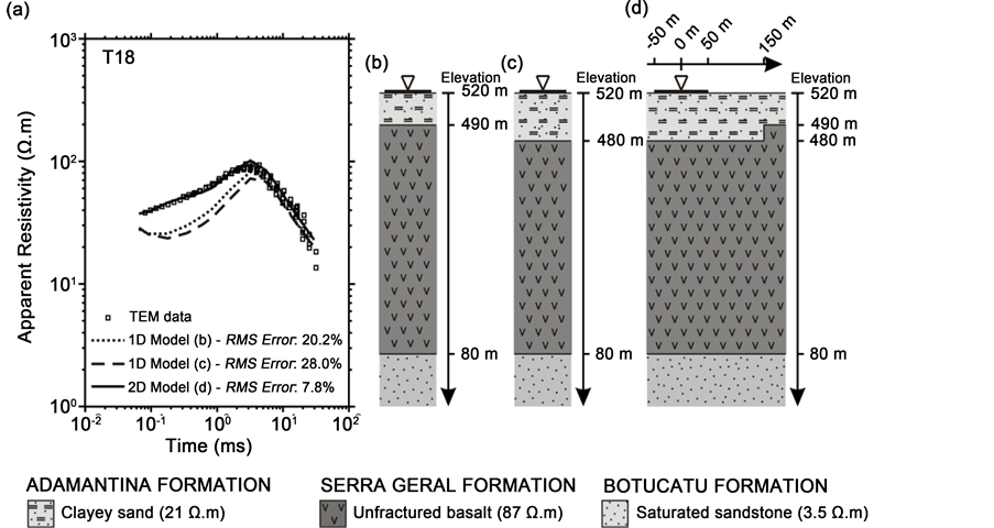
Figure 6. (a) Data curve and apparent resistivity curves modeled for the sounding T18. (b) 1D model with the clayey sand-basalt interface at 30 m deep. (c) 1D model with the clayey sand-basalt interface at 40 m deep. (d) 2D model with the clayey sand-basalt interface varying from 30 m to 40 m, 150 m away from the center of the sounding.
ble variation due to the geology (about 10 m only). The depth of 30 m shown for the same interface matches (also with an acceptable variation) with the top of the shallow resistive layer found in the 1D modeling from IX1D®v3.
Similar effects caused by lateral resistivity variation were observed in another 8 soundings. One of the most interesting is the T18 sounding with data curves and models shown in Figure 6. The 1D model from Figure 6(b) shows the interface between the sedimentary rocks and the basalt at 30 m deep, generating the synthetic result seen in Figure 6(a) (dotted curve). The clear discrepancy between this curve and the data curve before 4 ms and the fitting error of 20.2% indicate that this model cannot explain the data. Figure 6(c) shows a second 1D model, now with a 40 m deep interface. The synthetic response of this model generates lower apparent resistivity values, as expected from the analysis of the previous sounding, and increases the fitting error to 28.0%. A shallower depth for this interface is unacceptable, because it is not consistent with the geological information. In any event, there is no way to insert a simple horizontal interface that could explain such high apparent resistivity values.
To solve this problem, the 2D model presented in Figure 6(d) is proposed, which provides a good fit to the observed data (continuous curve in Figure 6(a)) with a small error of 7.8%. The lateral resistivity variation was modelled as a 10 m step located 150 m away from the center of the transmitter loop, and with depths varying from 30 m to 40 m, as shown in Figure 6(d). There are no exploitation wells near this sounding to compare with the geoelectrical model, but two other nearby soundings (T50 and T56) showed similar effects on their data curves and the elevation values for the top of the basalt layer is geologically compatible in all of them. The proposed distance between the step and the sounding center appears to be exaggerated, but there were no interference sources in the area that could cause such an effect on the data and lead to a wrong interpretation. There were some small brooks close by, but they did not have a sufficient amount of water to represent a significant interference source. Thus, the adoption of a 2D model may provide a possible explanation about the behavior of the data. The effects observed in this sounding are so strong that even the 2D model may be too simple to explain the lateral variations in the geology and maybe a 3D model may be required to better explain such distortion.
5. Discussion of Results
In addition to T68 and T18, the soundings T10, T37, T39, T50, T56, T69 and T74 also presented effects of lateral resistivity variation. Figure 7 and Figure 8 show the maps with the results for 2D modeling for these nine soundings. Since the models were made for each sounding individually, it is not possible to know where exactly the lateral resistivity variations are located. Hence, they are represented as dashed circles around each sounding center. The radius of each circle is equivalent to the distance between the center of the sounding and the step at the top of the basalt layer. Thus, the step at its upper interface can be placed anywhere over these circumferences. The crosses represent the location of TEM soundings that could be explained with a 1D model (as shown in Porsani et al. [17] while the crosses inside dashed circles represent the center of TEM soundings that were better explained using 2D models. The crosses with full white circles represent known exploitation wells. Crosses with full yellow circles are wells were abnormally high groundwater flow was observed. The normal

Figure 7. Topography of the basalt layer in Andes area and elevation values for soundings T10, T37, T39, T68, T69 and T74. Note that there are a concentration of 2D structures next to wells W07 and W10, which could explain the anomalous groundwater flow.

Figure 8. Topography of the basalt layer in Botafogo Area and elevation values for soundings T18, T50 and T56.
italic labels indicate the elevation of the interface between the Adamantina and Serra Geral Formations. The interpolated image in these figures represents the upper interface of the basalt layer. Each 1D model has only one elevation value for this interface, which is not shown in the figure for simplicity. On the other hand, as it is not possible to correctly locate the step in this interface due to limitation of the 2D analysis, each 2D model has two different labels for the interface elevation. One label refers to the elevation exactly below the center of the sounding and other label refers to the elevation far from its center. The topography of the interface between the Adamantina Formation and Serra Geral Formation was interpolated from 1D geoelectrical models obtained by Porsani et al. [17] , geological logs from the wells and from elevation values below the sounding center in 2D geoelectrical models.
Figure 7 shows the location of lateral resistivity variations modelled for soundings T10, T37, T39, T68, T69 and T74. The sounding T68 is the closest to a well, located at approximately 110 m from well W10. Its geoelectrical model shows the upper part of the interface between the Adamantina and Serra Geral Formations at an elevation of 515 m, which is in agreement with the results from the 2D model of sounding T69 and also with the elevation observed in the well W09 data log (507 m and 506 m respectively). The shallower part of the 2D model from sounding T68 shows this same interface at an elevation of 485 m, which conforms to W10 geological log data (Figure 3). The geoelectrical model suggests that there is a 30 m depth variation at the interface between these formations, which represents a considerable structuration at the top of the basalt layer. The sounding T39, located between wells W07 and W10, also shows a variation of 30 m in the interface depth, suggesting that a great structuration around these wells may also exist. The high groundwater flow rate reported at those wells can be related to such structures that might be intercepted during the drilling process. Sounding T39 is located a considerable distance from well W07 and it was not possible to allocate other TEM soundings closer to this well. Unfortunately, the ideal area for detailed surveys is located on private property and the access was denied to IAG/USP researchers. Sounding T74 is the only one to present lateral resistivity variation at the southern portion of the Andes area, with a vertical variation of 10 m located 70 m from the center.
The northern portion of the map shows a general decrease in the elevation from east to west, around soundings T10, T39, T68 and T69. The 2D models show that the elevation values at the center of the soundings are lower than those obtained through 1D modeling of surrounding soundings, but they are in conformance with the values observed in the wells. This suggests that these soundings are in an area with substantial structuration in the basalt layer. The effects in their respective data curves could be caused by independent structures or by one single, large structure. Considering the group of soundings T39, T68 and T69, one can observe that the decreasing topography is mainly in the SE-NW direction. This may be indicative that the steps in the interface are located in the southeastern portion of these three soundings, but it is not possible
to say if all the modelled steps are related to one single structure that would be aligned to the SW-NE direction. Despite this uncertainty, one can note that the variation around sounding T10 suggests a similar behavior for the subsurface structuration, i.e., it may be located also in its southeastern portion. In this sense, the structure could be placed from the southeastern portion to follow the decreasing in the SE-NW direction. Such comparison is more complicated for soundings T37 and T74 because there are no 1D models or wells nearby. In these cases, the step could be placed anywhere over the dashed circumference. Perhaps for T74 the structure would be placed also in its southeastern or eastern portion, which would also be in conformance with the structure location inferred for T10, T39, T68 and T69 from a regional point of view. However, it is difficult to reach such a conclusion because the vertical variation in T74 is just 10 m and there is no other sounding close to it that could show such effects for comparison. It is important to note that these six soundings are distributed around small brooks, which may be consequence of the probable structuration in subsurface.
Soundings T18, T50 and T56, located in the Botafogo area, form another group where some structuration influence was observed in the geoelectrical models. Figure 8 shows the topography map of the interface between the Adamantina and Serra Geral Formations containing them and other soundings with 1D models nearby. These three soundings are also located near a small brook, suggesting again that the existence of this drainage may be related to the existence of a structuration of upper interface of the basalt layer. Sounding T56 shows the greatest depth variation among all the 2D models studied. In this sounding the interface has a vertical variation of 40 m, which is located 60 m far from the sounding center. Sounding T50 has a vertical variation of 30 m, located 60 m far from the center.
One can observe on this map that the area around T18, T50 and T56 holds the minimum values of elevation, which is caused by the interpolation with the elevation values below the sounding center. As there is no sounding inside the imaginary triangle formed by these three soundings is difficult to infer a location for the vertical variation caused by the stepped structures. The only exploitation well available is located too far from the group to be helpful for this analysis. Nevertheless, one can observe that the elevation values in the center of soundings T50 and T56 are almost the same (464 m and 465 m respectively), suggesting that the variation in the elevation of these points may be very small. Looking to T18 and T56, one can see that the higher elevation values distant from the center of each sounding (490 m and 505 m respectively) may be comparable. In this sense, one possible interpretation is that the structures modelled for T18 and T56 would be located at the eastern portion of each sounding, while the structure modelled for T50 would be located at its western or southwestern portion. Comparing this to the brooks shown in the topography map of Figure 1 and considering that they are somehow related to structuration in subsurface, the southwestern portion may better for locating the structure in T50.
6. Conclusions
In this paper a study was carried out for geoelectrical mapping in an area with reported seismic activity. The study was done by means of several TEM soundings, of which nine were selected because they presented data curves affected by lateral resistivity variation effect and could not be well represented by 1D models. Then, those soundings were analyzed using a 2D modelling routine. The analyses have shown that all these soundings were under influence of some structuration at the upper interface of the basalt layer. This structuration was modeled as a step-like feature for each selected sounding.
The possible presence of a structuration between the sediments of Adamantina Fm. and the basalt of Serra Geral Fm. could be well-represented by the 2D TEM geoelectrical models. The fit between the data and the modelled response could be accomplished, as shown by the low fitting errors. The 2D modelling presented itself to be stable and efficient, with good applicability for detection of interface structuration. The modelling also allowed mapping the interface between a conductive layer over a resistive one, representing the inverse of an ideal scenario for TEM method.
All the soundings that showed the influence of a lateral resistivity variation are located near small brooks, observed in smooth valleys in the region. The presence of 2D structures near these features suggests that the local topographic variation may be conditioned to variations at the top of basalt layer.
The structures at the interface between the Adamantina and Serra Geral Formations may have been intercepted by the wells during the drilling process, providing a new connection between the shallow and the deep aquifers. It could possibly explain the anomalous groundwater flow at wells W07 and W10, suggesting a relation between the most structured areas and the foci of the seismic activities.
This sort of geoelectrical mapping would be useful for allocating groundwater wells at a region of interest. Moreover, knowing the existence of such structures can provide better models for the whole area, which might be used in other studies like for understanding the seismological processes occurring at that area. Those models could be used to provide additional information about the possible groundwater flow between the different aquifers present at the area. One limitation about the methodology used in this study is that the structuration could be placed at any point in a circumference around the sounding center, given a radius corresponding to the distance between the sounding center and the structuration. In order to improve this analysis a new survey could be done at the same area, with regular-spaced soundings along several parallel profiles. In this sense, the use of 3D modeling and inversion is suggested as an improvement to future research at this area. It would allow a more accurate location of the structures in the basalt layer in relation to TEM profiles and allow a better interpretation of the data sets, making possible the elaboration of a more plausible geoelectrical model for the studied area.
Acknowledgements
ERA thanks FAPESP-Fundação de Amparo à Pesquisa do Estado de São Paulo for the PhD scholarship (grants: 2011/21013-8 and 2013/12606-0). JLP acknowledges FAPESP for providing financial support for this research (2009/ 08466-3 and 2012/15338-4), and CNPq-Conselho Nacional de Desenvolvimento Científico e Tecnológico for providing a research grant (301692/2013-0 and 406653/2013-5), both are Brazilian research agencies. IAG/USP is also acknowledged for providing infrastructure support. We thank Ernande, Marcelo, David, Vinícius, Divanir, Rodrigo, Tiago and other students for helping us during the campaigns for data acquisition. We also thank to Professor Dr. Scott Joseph Allen (UFPE) for his corrections and suggestions in the text.
Cite this paper
Almeida, E.R., Porsani, J.L., dos Santos, F.A.M. and Bortolozo, C.A. (2017) 2D TEM Modeling for a Hydrogeological Study in the Paraná Sedimentary Basin, Brazil. International Journal of Geosciences, 8, 693-710. https://doi.org/10.4236/ijg.2017.85038
References
- 1. Fitterman, D.V. and Stewart, M.T. (1986) Transient Electromagnetic Sounding for Groundwater. Geophysics, 51, 955-1005.
https://doi.org/10.1190/1.1442158 - 2. McNeill, J.D. (1994) Principles and Application of Time Domain Electromagnetic Techniques for Resistivity Sounding. Technical Note TN-27, Geonics Ltd., Ontario.
- 3. Krivochieva, S. and Chouteau, M. (2003) Integrating TDEM and MT Methods for Characterization and Delineation of the Santa Catarina Aquifer (Chalco Sub-Basin, Mexico). Journal of Applied Geophysics, 52, 23-43.
https://doi.org/10.1016/S0926-9851(02)00231-8 - 4. Ezersky, M., Legchenko, A., Al-Zoubi, A., Levi, E., Akkawi, E. and Chalikakis, K. (2011) TEM Study of the Geoelectrical Structure and Groundwater Salinity of the Nahal Heversink Hole Site, Dead Sea Shore, Israel. Journal of Applied Geophysics, 75, 99-112.
https://doi.org/10.1016/j.jappgeo.2011.06.011 - 5. Land, A.L., Lautier, J.C., Wilson, N.C., Chianese, G. and Webb, S. (2003) Geophysical and Monitoring Evaluation of Coastal Plain Aquifers. Ground Waters, 42, 59-67.
https://doi.org/10.1111/j.1745-6584.2004.tb02450.x - 6. Nielsen, L., Jorgensen, N.O. and Gelting, P. (2007) Mapping of the Freshwater Lens in a Coastal Aquifer on the Keta Barrier (Ghana) by Transient Electromagnetic Soundings. Journal of Applied Geophysics, 62, 1-15.
https://doi.org/10.1016/j.jappgeo.2006.07.002 - 7. Christiansen, A.V., Auken, E. and Sorensen, K. (2006) The Transient Electromagnetic Method. In: Kirsch, R., Ed., Groundwater Geophysics—A Tool for Hydrogeology, GSW Ltd., Aarhus, 179-225.
- 8. Danielsen, J.E., Auken, E., Jorgensen, F., Sondergaard, V. and Sorensen, K.I. (2003) The Application of the Transient Electromagnetic Method in Hydrogeophysical Surveys. Journal of Applied Geophysics, 53, 181-198.
- 9. Jorgensen, F., Sandersen, P.B.E. and Auken, E. (2003) Imaging Buried Quaternary Valleys Using Transient Electromagnetic Method. Journal of Applied Geophysics, 53, 199-213.
https://doi.org/10.1016/j.jappgeo.2003.08.016 - 10. Santos, F.A.M. and El-Kaliouby, H. (2011) Quasi-2D Inversion of DCR and TDEM Data for Shallow Investigations. Geophysics, 76, F-239-250.
https://doi.org/10.1190/1.3587218 - 11. Teatini, P., Tosi, L., Viezzoli, A., Baradello, L., Zecchin, M. and Silvestri, S. (2011) Understanding the Hydrogeology of the Venice Lagoon Subsurface with Airborne Electromagnetic. Journal of Hydrology, 411, 342-354.
https://doi.org/10.1016/j.jhydrol.2011.10.017 - 12. Martínez-Moreno, F.J., Santos, F.A.M., Madeira, J., Bernardo, I., Soares, A., Esteves, M. and Adão, F. (2016) Water Prospection in Volcanic Islands by Time Domain Electromagnetic (TDEM) Surveying: The Case Study of the Islands of Fogo and Santo Antão in Cape Verde. Journal of Applied Geophysics, 134, 226-234.
https://doi.org/10.1016/j.jappgeo.2016.09.020 - 13. Meju, M.A., Fontes, S.L., Oliveira, M.F.B., Lima, J.P.R., Ulugergerli, E.U. and Carrasquilla, A.A.G. (1999) Regional Aquifer Mapping Using Combined VES-TEM-AMT-EMAP Methods in the Semi-Arid Eastern Margin of Parnaiba Basin, Brazil. Geophysics, 64, 337-356.
https://doi.org/10.1190/1.1444539 - 14. Carrasquilla, A.A.G. and Ulugergerli, E. (2006) Evaluation of the Transient Electromagnetic Geophysical Method for Stratigraphic Mapping and Hydrogeological Delineation in Campos Basin, Brazil. RevistaBrasileira de Geofísica, 24, 333-341.
https://doi.org/10.1590/S0102-261X2006000300003 - 15. Santos, H.S. and Flexor, J.M. (2008) O Método Transiente Eletromagnético (TEM) Aplicado Ao Imageamento Geoelétrico Da Bacia de Resende (RJ, Brasil). RevistaBrasileira de Geofísica, 26, 543-553.
https://doi.org/10.1590/S0102-261X2008000400013 - 16. Porsani, J.L., Bortolozo, C.A., Almeida, E.R., Sobrinho, E.N.S. and Santos, T.G. (2012) TDEM Survey in Urban Environmental for Hydrogeological Study at USP Campus in São Paulo City, Brazil. Journal of Applied Geophysics, 76, 102-108.
https://doi.org/10.1016/j.jappgeo.2011.10.001 - 17. Porsani, J.L., Almeida, E.R., Bortolozo, C.A. (2012) TDEM Survey in an Area of Seismicity Induced by Water Wells in Paraná Sedimentary Basin, Northern São Paulo State, Brazil. Journal of Applied Geophysics, 82, 75-83.
https://doi.org/10.1016/j.jappgeo.2012.02.005 - 18. Bortolozo, C.A., Porsani, J.L., Santos, F.A.M. and Almeida, E.R. (2015) VES/TEM 1D Joint Inversion by Using Controlled Random Search (CRS) Algorithm. Journal of Applied Geophysics, 112, 157-174.
https://doi.org/10.1016/j.jappgeo.2014.11.014 - 19. Bortolozo, C.A., Couto, M.A., Porsani, J.L., Almeida, E.R. and Santos, F.A.M. (2014) Geoelectrical Characterization Using Joint Inversion of VES/TEM Data: A Case Study in Paraná Sedimentary Basin, São Paulo State, Brazil. Journal of Applied Geophysics, 111, 33-46.
https://doi.org/10.1016/j.jappgeo.2014.09.009 - 20. Campana, J.D.R., Porsani, J.L., Bortolozo, C.A., Oliveira, G.S. and Santos, F.A.M. (2017) Inversion of TEM Data and Analysis of the 2D Induced Magnetic Field Applied to the Aquifers Characterization in the Paraná Basin, Brazil. Journal of Applied Geophysics, 138, 233-244.
https://doi.org/10.1016/j.jappgeo.2017.01.024 - 21. Bortolozo, C.A. (2016) 1D and 2D Joint Inversion of Electroresistivity Data and TEM Applied in Hydrogeology Studies in the Paraná Basin. Ph.D. Thesis, Universidade de São Paulo, Sao Paulo.
- 22. Bortolozo, C.A., Campana, J.D.R., Couto Jr., M.A., Porsani, J.L. and Santos, F.A.M. (2016) The Effects of Negative Values of Apparent Resistivity in TEM Surveys. International Journal of Geosciences, 7, 1182-1190.
https://doi.org/10.4236/ijg.2016.710088 - 23. Interpex (2008) IX1D v3 Instruction Manual. Interpex Ltd., 1-133.
- 24. Assumpção, M., Yamabe, T., Barbosa, J.R., Hamza, V., Lopes, A.E.V., Balancin, L. and Bianchi, M.B. (2010) Seismic Activity Triggered by Water Wells in the Parana Basin, Brazil. Water Resources Research, 46, Article ID: W07527.
https://doi.org/10.1029/2009wr008048 - 25. Giampá, C.E.Q. and Souza, J.C. (1982) Potencial Aquífero Dos Basaltos Da Formação Serra Geral No Estado de São Paulo.2 Congresso Brasileiro de águasSubterraneas, Anais, 42, 3-15.
- 26. Oristaglio, M.L. and Hohmann, G.W. (1984) Diffusion of Electromagnetic Fields into a Two-Dimensional Earth: A Finite-Difference Approach. Geophysics, 49, 870-894.
https://doi.org/10.1190/1.1441733