International Journal of Geosciences
Vol.07 No.06(2016), Article ID:67912,24 pages
10.4236/ijg.2016.76063
Three-Dimensional Shear Wave Velocity Structure of the Northeastern Brazilian Lithosphere
Jorge Luis de Souza1*, Newton Pereira dos Santos1, Carlos da Silva Vilar1,2
1Coordenação de Geofísica, MCTI/Observatório Nacional, Rio de Janeiro, Brazil
2Departamento de Física da Terra e do Meio Ambiente, Universidade Federal da Bahia (UFBA), Brazil

Copyright © 2016 by authors and Scientific Research Publishing Inc.
This work is licensed under the Creative Commons Attribution International License (CC BY).
http://creativecommons.org/licenses/by/4.0/


Received 20 May 2016; accepted 27 June 2016; published 30 June 2016
ABSTRACT
A large number of Rayleigh wave dispersion curves recorded at twenty three seismic stations was used to investigate the 3-D shear wave velocity structure of the northeastern Brazilian lithosphere. A simple procedure to generate a three-dimensional image of Mohorovičić discontinuity was applied in northeastern Brazil and the Moho 3-D image was in agreement with several isolated crustal thicknesses obtained with different geophysical methods. A detailed 3-D S wave velocity model is proposed for the region. In the crust, our model is more realist than CRUST2.0 global model, because it shows more details either laterally or in depth than global model, i.e., clear lateral variation and gradual increase of S wave velocity in depth. Down to 100 km depth, the 3-D S wave velocity model in northeastern Brazil is dominated by low velocities and this is consistent either with heat flow measurements or with measurements of the flexural strength of the lithosphere developed in the South American continent. Our 3-D S wave velocity model was also used to obtain the lithosphere thickness in each cell of the northeastern Brazil and the results were consistent with global studies about the Lithosphere-Asthenosphere Boundary worldwide.
Keywords:
Rayleigh Waves, Group-Velocity Tomography, Three-Dimensional Shear Wave Velocity, Lithosphere, Spatial Resolution, Northeastern Brazil

1. Introduction
The small quantity and the poor distribution of seismic stations in the Brazilian territory can be considered the major factors for the poor knowledge of the earth’s interior in the last decades. The major part of the regional surface wave investigations in Brazil and surrounding areas ( [1] - [6] ) has been made through reduced quantity of dispersion data along large source-station paths, where surface waves cross several different geological provinces and the estimated S wave velocity structure varies only in depth (i.e. only a few 1-D profiles).
The recent installation of modern seismic stations in the South America continent, as initiative of international institutions (IRIS, GEOFON, GEOSCOPE, etc.) and, mainly, with the seismic data available to the seismological community, has allowed the development of more detailed studies about the earth’s interior in Brazil. The free access to those high quality seismic data has allowed the development of some 3-D shear wave velocity studies in both southeastern and northeastern Brazil ( [7] - [10] ).
In the recent years, the general aspects of the shear wave velocity structure of the South America continent has been studied via surface waves ( [11] - [14] ). In some cases, the investigation was concentrated in specific areas of the continent, such central and western South America ( [11] ). In this study, they used waveform of Rayleigh waves to image the 3-D S wave velocity structure of the region. The general features of four slices (at 100, 150, 200 and 300 km depth) of the proposed model for the region were presented and discussed. The spatial resolution of this study was obtained through resolution tests (based essentially on synthetic data with random noise) and it was qualitatively classified into very good (to depths above 300 km) and none to good (to depths below to 300 km). In other study in the South America continent, [12] used both Rayleigh (from 10 to 150 s) and Love waves (from 20 to 70 s) group-velocities to analyze the 3-D S-velocity structure of the region. In this case, the region was discretized into cells of 2˚ × 2˚ and the problem was solved via conjugate-gradient method. A regionalized dispersion curve at each cell of the grid was then used to estimate the 1-D S-velocity in depth. The spatial resolution was obtained through both checkerboard and realistic structure tests. According to [12] , the spatial resolution at 30 km is around 4˚, while at 100 km it is 6˚ and at 150 km it is 8˚. The general features of the S wave velocities anomalies at those depths were presented and discussed. More recently, [13] used joint inversion of waveform and fundamental mode Rayleigh wave group-velocities to investigate the South America continent. The methodologies used by both [12] and [11] were used in this study to get group-velocities and waveform inversions, respectively. The spatial resolution was obtained with checkerboard tests and according to the authors it was 6˚ at both 100 and 300 km depths. The S wave velocities anomalies to these depths were presented and discussed. The most recent study about the S wave velocity structure beneath South America continent was presented by [14] . He used a group of 128 earthquakes occurred at western South America continent and recorded by 71 seismic stations distributed throughout continental part of the region. Rayleigh wave group-velocities varying from 5 to 250 s were used to obtain the source-station dispersion curves. The region was divided into cells of 4˚ × 4˚ and a regionalized Rayleigh wave dispersion curve was obtained for each cell of the grid. Each regionalized dispersion curve was inverted to get a 1-D S wave velocity in each cell. None evaluation about spatial resolution (either qualitative or quantitative) of the estimated shear wave velocity in the region is presented. Only a qualitative evaluation of the resolution (i.e., the terms bad resolution and poor resolution are applied to classify the resolution in depth) is presented and discussed.
Our objective is to present the results of a detailed 3-D shear wave velocity structure study in northeastern Brazil. It is well known, in the seismological literature, that a 3-D shear wave velocity structure study, via surface waves, is commonly divided into two main steps. In the first step, the source-station dispersion curves are used in a 2-D inversion process (i.e., a regionalization process or a phase and/or group-velocity tomography) to get a dispersion curve representative of each element of the total area (i.e. a cell). In the second step, the dispersion curve of each cell is used in a 1-D inversion process to obtain the shear wave velocity structure in depth, so that a 3-D S wave velocity model of the region can be constructed from the spatial representation of those 1-D inversions.
In this study, a large quantity of Rayleigh wave group-velocities, recorded at several seismic stations of Incorporated Research Institutions for Seismology (IRIS) Consortium, was used to investigate the 3-D shear wave velocity structure of the northeastern Brazilian lithosphere. The methodology used in the estimation of the Rayleigh wave group-velocities in northeastern Brazil is presented in the Section 2. In Section 3, both data and its processing, to get the dispersion curves from source to station, are presented and discussed. The Section 4 is dedicated to the quantitative analysis of the spatial resolution of the regionalized Rayleigh wave group-velocities, which are directly related to the estimated shear wave velocity structure in northeastern Brazil. In both Sections 5.1 and 5.2, respectively, a 3-D image of Mohorovičić Discontinuity and the 3-D shear wave velocity structure of northeastern Brazil are proposed and analyzed in detail, by using previous studies available in the seismological literature. The main conclusions of our study are condensed in Section 6.
2. Two-Dimensional Surface Wave Tomography
Estimation of the Rayleigh Wave Group-Velocities in Northeastern Brazil
The region limited by the geographical coordinates (−125, 45) and (25, −75) is, initially, divided into square cells of 2˚ × 2˚ (Figure 1). Let’s consider that there are m source-station Rayleigh wave paths crossing the target area (Figure 1) and also assume that for a particular path, the total source-station Rayleigh wave travel time is the sum of the travel time in each cell. Thus, for an ith path and a given period (T), we can write ( [15] )
 (1)
(1)
where vj(T) is an attributed group-velocity for the jth cell, Vi(T) is the source-station group-velocity for the ith path calculated from attributed vj(T), Ui(T) is the observed source-station group-velocity for the ith path, uj(T) is the group-velocity for the jth cell, dij is the length of the ith path in the jth cell, and Di is the source-station distance of the ith path.
At this time, a relevant point, which is related to the computation of both partial and total source-station distances (i.e., the terms dij and Di in Equation (1)) should be cited. In this case, to obtain precise partial and total source-station distances, an ellipsoidal earth model and Rudoe’s formula were applied ( [16] ).
Our objective is to estimate the group-velocity for each cell of Figure 1, i.e. the term uj(T), by using the Equation (1). Thus, for a particular period (T), the following procedures were applied in the solution of the equation system:
1―To get the best solution of the equation system (1), a group-velocity range (Δc) covering a large interval of group-velocities (cn,  iterations) and a group-velocity step (ζ) are previously defined;
2―The first value of the group-velocity range (i.e., a constant group-velocity value?c1) is then attributed in all cells of the grid (vj values);
3―With the vj values of the previous item, the Vi values are then calculated;
4―As the terms Ui, dij and Di are known, then the equation system is solved (for the particular group-velocity c1?item 2) and the values of uj are computed via Equation (3). In this step, both resolution and covariance matrices are also computed by using Equations (4) and (5);

Figure 1. Seismic stations (red triangles) and epicenters of the earthquakes (blue circles) used in the present study. The area is limited by the geographical coordinates (−125, 45) and (25, −75). The heavy square box represents the target area, i.e., northeastern Brazil.
5―With the uj values obtained in the previous step, the source-station travel times for all paths are then calculated and they are compared with the observed source-station travel times, so that a set of time residuals (tri) is estimated and a root mean square of those values is calculated and storage in a vector (qn,  iterations);
6―The next value of the group-velocity range (i.e., c2 = c1 + ζ) is attributed and the whole process starts again, i.e., it goes to step 3;
7―When the group-velocity range (Δc) is completed (p iterations), the set of root mean square values storage in the item 5 (vector qn) is used to find the minimum one or the best solution of the tomographic problem.
The result of the procedure aforementioned is a Rayleigh wave dispersion curve for each cell of Figure 1. It is also important to remember that only the cells visited by at least one Rayleigh wave path are considered in such computation. Equation (1) can be rewritten in a matrix form as
 (2)
(2)
where y is a residual vector (m ´ 1), x is a vector with the unknown parameters (n ´ 1) and A is a m ´ n matrix relating model parameters to observations. In terms of damped least-squares ( [17] [18] ), Equation (2) is given by
 (3)
(3)
where AT is the transpose of matrix A,  is the Levenberg-Marquardt parameter, and I is the identity matrix. In this context, the expressions for resolution (R) and covariance (C) matrices are the following
 (4)
(4)
 (5)
(5)
where σ2 is the variance in the observations. The standard deviations of the estimated group-velocities at each cell of the northeastern Brazil are obtained in the diagonal elements of the covariance matrix. Furthermore, several factors can contribute to uncertainties in group-velocity estimation ( [19] ). These include origin time error, epicenter mislocation error, source finiteness error, rise time error, etc. These errors were estimated and incorporated to the σ2 term of the covariance matrix (C).
As our goal is to investigate northeastern Brazil (Figure 1), thus we selected only the Rayleigh wave dispersion curves associated with each cell of such region (Figure 2). For each period, its source-station Rayleigh wave path distributions were plotted into maps to have an idea about their spatial distribution. Some of those maps are shown in Figure 3.

Figure 2. The grid of the Figure 1 was divided into cells of 2˚ × 2˚ and each cell on it was numbered (from top to bottom and from left to right) so that any region inside northeastern Brazil must be associated with the numbers shown on the map.


Figure 3. Source-station Rayleigh wave path distributions (for ten periods) in the area of the northeastern Brazil. The black lines are the great-circle paths connecting epicenters and stations. The target area is relatively well covered by the Rayleigh wave path distribution. The maps show a clear decrease in the quantity of the source-station paths, when the period increases.
3. Data Processing
In order to have a good path coverage of the target are (i.e. northeastern Brazil), a large quantity of earthquakes recorded at twenty three seismic stations (from 1988 to 1998 [10] ) of the IRIS Consortium ( [20] ), located either in or around South America continent, were selected in this study (Figure 1).
Many digital seismograms, related to seismic events with focal depth shallower than 120 km and magnitude higher than 5.0 mb, were requested and received from IRIS. The Seismic Analysis Code (SAC) package ( [21] ) was used to the identification of the surface waves in the seismic signals. This analysis produced 3134 digital seismograms, corresponding to 1082 earthquakes (Figure 1). The vertical components of the motion were used here and they represent 3134 source-station Rayleigh wave paths in the area displayed in Figure 1. To remove the effect of the seismograph on the seismic signal, a instrumental correction was applied in the seismograms (via SAC). Correction for source group delay was not applied, because it is considered a small source of error ( [22] ). The Multiple-Filter Technique ( [23] ) was applied in the digital seismograms selected for this study.
Twenty two periods, ranging from 10 to 102s (i.e., 10.04, 12.05, 14.03, 16.00, 18.29, 20.08, 24.38, 28.44, 32.00, 36.57, 42.67, 46.55, 51.20, 56.89, 60.24, 64.00, 68.27, 73.14 78.77, 85.33, 93.09 102.40s), were selected to compose the source-station dispersion curves. This computation produced 3134 source-station Rayleigh wave group-velocity dispersion curves. In the next section, these dispersion curves are used to get a dispersion curve representative of each element of the total area (i.e., a cell of 2˚ × 2˚).
4. Resolution of the Group-Velocities in Northeastern Brazil
In this study, the methodology proposed by [24] is used to analyze the resolution of the estimated group- velocities in northeastern Brazil. In such approach, the resolution at any cell of a gridded region is given by
 (6)
(6)
where c is a parameter obtained after two main procedures, i.e., a linearization of the estimated resolving kernels (Equation (4)) followed by a quadratic least-squares fit ( [24] ). W is a quantitative spatial resolution measurement of the unknown parameter (in this case, it is the estimated Rayleigh wave group-velocity either at a specific cell or at a particular period).
The Equation (6) was used to get the spatial resolution of the estimated Rayleigh wave group-velocities at each cell of the northeastern Brazil. As the region under investigation is formed by 49 cells (Figure 2) and each cell has a dispersion curve (which is composed of 22 periods), we got 1078 resolution estimates (49 × 22) for the northeastern Brazilian region. All those results are condensed in Table 1. For a given cell of the northeastern Brazilian region, we got five elements of the resolution matrix (Equation (4)). The central point (third element) is related to the center of the cell under evaluation and the others four points are located in the centers of the neighborhood cells (two on left and two on right). Here, the separation between each central point is equal to 2˚, because the studied area was divided into cells of 2˚ × 2˚, thus the separation between the five points is equal to 2˚.
A few cases displayed in Table 1 are used in Figure 4 to show the procedure to estimation of the spatial resolution at each cell in the northeastern Brazil. First, the five elements of the resolving kernel at a particular cell (and for a specific period) are used to calculate the parameter c and it is used in Equation (6) to estimate the spatial resolution at this particular cell and period ( [24] ). The black circles are the five elements of the resolution matrix (the resolving kernel computed from Equation (4)) for a specific cell and period. They are located at 2, 4, 6 (third element or central point), 8 and 10 positions. As mentioned previously, they are separated by 2˚, because of the cell size in the 2-D inversion process. The red square is the theoretical Gaussian function calculated with the Gaussian fit coefficients. In the upper right side is shown the spatial resolution (W-Equation (6)) and the Correlation Coefficient (CC) between the resolving values and the theoretical Gaussian function calculated with the Gaussian fit coefficients. An analysis of the correlation coefficients values displayed in Table 1 shows that 70% of them are equal and higher than 0.7. It shows that the Gaussian function seems to be a good representation of the resolving kernels’ shape.
The results displayed in Table 1 also show some interesting features. First, the spatial resolution in northeastern Brazil (Figure 2) spreads over a wide range from 3.2˚ to 12.7˚, but the major part of them is concentrated between 4.0˚ and 8.0˚, i.e., from two to four cells. This spatial resolution range is in agreement with all previous tomographic and 3-D shear wave velocities studies developed in the South American continent ( [25] ―8˚; [26] ―from 6˚ to 9˚; [27] ―5˚; [12] ―from 4˚ to 8˚; [13] ―6˚). Second, Table 1 indicates that the group- velocity anomalies (or shear wave velocity anomalies) smaller than 3.2˚ cannot be resolved in northeastern Brazil and, therefore, such anomalies should not be considered in the analysis of the results. As each period (or frequency) of the surface waves is related to a sampled region in depth, thus the method proposed by [24] allows to analyze any Rayleigh wave group-velocity anomaly (or shear wave velocity anomaly) in any particular point of the 2-D area, along the depth range covered by the dispersion curves.
Despite the fast reduction in the Rayleigh wave paths quantity in NE Brazil, when the period increases (Figure 3), the spatial resolution value for a given cell varies smoothly and this behavior is compatible with the depth sampled by the seismic surface waves during the propagation from source to station. In general, the spatial resolution becomes smaller when the period increases and it is probably associated with a better Rayleigh wave path coverage in the region (Figure 3). As expected, for the spatial resolution, we believe that the surface wave path distribution should be more important than the quantity of source-station Rayleigh wave paths.
Furthermore, our spatial resolution range is also in agreement with the theoretical restrictions associated with the influence zone or the first Fresnel zone, which is defined as an area (around a surface wave path) where surface wave phases are coherent and there is only constructive interference from scattered waves ( [28] ). In geometrical ray theory, which is based on high-frequency approximation, the influence zone around a surface wave

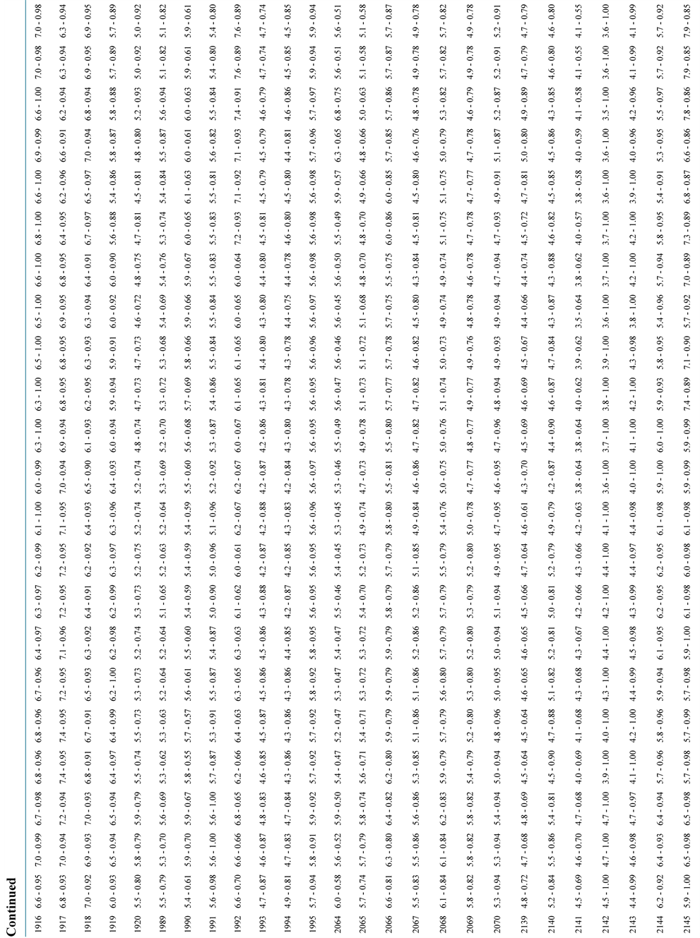
Table 1. Estimated spatial resolutions (in degrees) for each cell of the northeastern Brazilian region obtained via Gaussian fit. The numbers behind the spatial resolutions are the correlation coefficients between the resolution values, estimated via resolution matrix (Equation (4)), and those computed with Gaussian fit coefficients. To analyse the distinct aspects of the spatial resolutions throughout the grid, at a particular place, the midpoint of the resolution values (i.e., spatial resolution/2) should be placed in the center of the cell. This table shows the estimated resolutions for all cells of northeastern Brazil (Figure 2) and for all periods of the dispersion curves. An important feature observed in the estimated resolutions is the global spatial range, which varies from 3.2˚ to 12.7˚, but the major part of them is concentrated between 4.0˚ and 8.0˚ (i.e., from two to four cells). The large quantity of correlation coefficients higher than 0.7 (70%) indicates that a Gaussian function is a good representation of the resolving kernels’ shape.


Figure 4. Examples of spatial resolution estimates at some cells and periods displayed in Table 1 ( [24] ). The black circles are the five elements extracted from the resolution matrix (Equation (4)) at a particular cell (central element―position 6) and period. The red squares are the theoretical values computed with the coefficients of the Gaussian fit. In the upper left side the legend of the symbols (res―resolving values from resolution matrix and gau―theoretical Gaussian values). In the upper right side, one can find both the estimated spatial resolution value (W), for a specific cell, and the correlation coefficient (CC) between the resolving values from resolution matrix and the theoretical values calculated with the coefficients of the Gaussian fit. In all cases, the theoretical Gaussian curve is very close to the estimated resolution value obtained with the resolution matrix. This is confirmed by the high quantity of correlation coefficients in Table 1. It suggests that a Gaussian function represents very well the resolving kernels’ shape.
source-station path is supposed to be like a delta function. Nevertheless, actual surface waves with finite frequency sample a finite region around a ray path (physical ray [28] ). According to [29] , the maximum width (LF) of the first Fresnel zone (in radians) is given by the following expression
 (7)
(7)
where λ is the wavelength (in radians) and Δ is the epicentral distance. Equation (7) shows that Fresnel’s zones width increases with increasing wavelength and epicentral distance. According to [28] , the estimated width of the influence zone is approximately one-third of the first Fresnel zone (LF/3).
In order to investigate Fresnel’s zone width in this study, we considered the data set associated with two periods (10.04 s and 102.40 s). The epicentral distances of the Rayleigh wave paths that crossed northeastern Brazilian region were classified into several distinct classes (Figure 5). In both cases, the epicentral distances spread over a wide range, which varies mainly from 20˚ to 120˚, but they are concentrated around 70˚ (Figure 5). An important feature to be observed in Figure 5 is that the major part of the source-station distances (66% either to 10.04 s or to 102.40 s) is less than 80˚. It means that the group-velocity estimates are mainly influenced by those Rayleigh wave source-station paths and, therefore, their Fresnel’s zone width should have a higher weight in the process than the other source-station paths. The width of the influence zone, for both minimum and maximum periods considered in the group-velocity estimation, is displayed in Table 2. It shows that for epicentral distances ranging from 20˚ to 120˚, our spatial resolution range estimates are in the same range of the influence zone predicted by the geometrical ray theory.


Figure 5. Number of source-station Rayleigh wave paths in the northeastern Brazil (as a function of epicentral distance), divided into seven classes. It shows that the major part of the surface wave paths (66%) has epicentral distance lower than 80˚.

Table 2. One-third of the first Fresnel’s zone width (LF/3) calculated with Equation (7), by using the minimum and maximum periods (T) of the dispersion curves in northeastern Brazil. Δ is the epicentral distance and c is the phase velocity of PREM. Our spatial resolution range estimates (from 4˚ to 8˚) are compatible with the influence zone of the physical ray, as defined by [28] .
5. Results and Discussions
5.1. Three-Dimensional Image of Mohorovičić Discontinuity in Northeastern Brazil
In order to understand the dynamics of several geological processes (i.e., mountain ranges, subduction, rifting and basin formation) it is fundamental to have information about crustal thickness in distinct geotectonic provinces. Seismic reflection and refraction data are the best way of getting both precise and reliable determinations of such parameter. However, in general, the practical procedures to obtain those data are very expensive. In this context, surface wave data can be an inexpensive alternative way to get information about crustal thickness in any place of the world.
In the recent years, surface wave data (dispersion and waveform) have been used to provide information about crustal thickness in the earth’s interior. The major part of those studies is based on Genetic Algorithms (GA) applied into local and regional surface wave waveform ( [30] [31] ) and inter-station dispersion curves ( [32] ). These methods make a direct comparison between theoretical and observed variables in large data sets (large quantity of earth models) to find a particular population, where the misfit reaches an acceptable range. In addition, Grid Search (GS) technique has also been applied into dispersion data to get information about crustal thickness in the earth’s interior ( [33] [34] ). As well as GA, the GS technique applies the same procedures, described previously, to find a solution for the problem.
Two important points must be observed in the procedure adopted in this study. First, each dispersion curve is sensitive to the lithosphere structure beneath the area that it represents (i.e. a cell) and the period range of the dispersion curve (from 10 to 102 s) is suitable for identification of Mohorovičić Discontinuity (MD) depth. Second, for a dispersion curve (i.e., a dispersion curve which should be, theoretically, strongly affected by local shear wave velocity in depth) a S wave velocity contrast at MD depth is out of question remarkable, and such information is certainly present in the dispersion data.
A simple procedure, which can be summarized into two main steps well consolidated in the surface wave studies, defines the methodology used in this study to generate the 3-D image of Mohorovičić Discontinuity in northeastern Brazil. In the first step, the source-station Rayleigh wave group-velocities are used in a 2-D inversion process in order to get a dispersion curve representative of each cell of the NE Brazilian region. In the second step, the dispersion curve of a given cell is 1-D shear wave velocity inverted many times (i.e. a dispersion curve for such cell is inverted for a limited quantity of crustal models, where the thickness of the models varies from thin to thick) to find the best fit between observed and theoretical dispersion curves. The best fit, which is characterized by the minimum Root Mean Square (RMS) between observed and theoretical Rayleigh wave group velocities, provides both the S wave velocity structure in depth and its corresponding crustal thickness of such cell.
The first step was described, in detail, in the section 3. Therefore, the dispersion curves in each cell of the northeastern Brazil are ready to be used. It should be noted that the target area is composed of three types of cells (Figure 2), i.e., purely continental, purely oceanic and mixed (both continental and oceanic parts), and for each cell we have a dispersion curve representative of it. Thus, if the cell is continental, the dispersion curve is inverted (for S wave velocities in depth) 69 times (i.e., 69 different crustal models and crustal thicknesses). If the cell is oceanic, the dispersion curve is inverted (for S wave velocities in depth) 150 times (i.e., 150 different crustal models and crustal thicknesses). In the mixed cells, the dispersion curve is inverted 219 times (69 crustal models for the continent and 150 crustal models for the ocean parts). It must be noted that a dispersion curve is inverted and not compared with a theoretical one generated by a forward modeling, such as applied in both GA ans GS techniques.
In the continent, we generated 69 crustal models, by combining layers of the upper crust (2, 3, 4, 5, 6, 7, 8, 9, 10, 15 or 20 km thickness) with layers of the lower crust (5, 10, 15 or 20 km thickness), so that each crustal model has a distinct crustal thickness. In the ocean, we generated 150 crustal models, by combining layers of water (1, 2, 3, 4 or 5 km thickness), layers of sediments (0.5, 1, 2, 4, 6, or 8 km thickness) and layers of lower crust (2, 4, 6, 8, or 10 km thickness), so that each crustal model has a different crustal thickness. The above combinations allow for crustal thickness varies from 18 to 66 km (in the continent) and from 3.5 to 23 km (in the ocean). The upper mantle is common for both continental and oceanic structures and it is represented by eight layers of 20 km thickness, and the layer thicknesses are fixed during dispersion inversion. Thus, only S wave velocities in depth are inverted in the upper mantle. Examples of crustal models used in the dispersion inversion procedures are shown in Table 3.
To estimate the S wave velocity structure in depth, at each cell of the target area (Figure 2), we used SURF package ( [35] ). It has been widely used in surface wave dispersion studies worldwide ( [3] [4] , [36] - [38] ). Both P and S wave velocities, as well as density of Preliminary Reference Earth Model ( [39] ) were used as starting parameters in the dispersion inversion procedure.
In conclusion, our procedure looks for the best combination of crustal S wave velocities layers in depth through a simple RMS value between theoretical and observed dispersion curves in a given cell. Thus, for a particular cell, the dispersion curve is then inverted (69, 150 or 219 times) and the minimum Root Mean Square (RMS) between observed and theoretical Rayleigh wave dispersion curves is identified to find its corresponding S wave velocity structure in depth and crustal thickness.
An example of this procedure for a continental cell (corners (−39, −5) and (−37, −7)―Figure 2) is displayed in Figure 6. It is clear that there are two different levels of RMS and that a transition zone occurs between crustal models 45 and 50. It is also possible to observe two different scatter zones in both sides of the transition zone, i.e., the first scatter zone is stabler than the second one (Figure 6). In fact, crustal models from 1 to 51 are represented by intermediate and thick crustal thicknesses (first scatter zone―Figure 6), whereas the crustal models from 52 to 69 are characterized by thin crustal thicknesses (second scatter zone―Figure 6). As the results shown in Figure 6 are referred to a continental cell, thus we expect a stable behavior in the first scatter zone, as well as a lowest RMS level and consequently the minimum RMS value. These features are clearly observed in Figure 6.
The methodology described previously was applied at each cell of the northeastern Brazil (Figure 2) and the results produced two types of information, i.e., the MD thickness (the lowest RMS between observed and theoretical dispersion curve) and its corresponding S wave velocity structure in depth. Thus, the first information

Figure 6. The Root Mean Square (squares) of the sixty nine Rayleigh wave group-velocity dispersion inversions, for a continental cell (corners at (−39, −5) and (−37, −7)―Figure 2), shows a few interesting aspects. Two levels of RMS scatters are observed and they have different DC levels. Arrow indicates the minimum RMS, and corresponding crustal model has 28 km thickness. This value is the same than that found by [41] using seismic refraction methods. Absence of squares means that RMS is larger than 0.1 km/s.
Table 3. Examples of Earth models used in the generation of the 3-D image of Moho discontinuity (Section 5.1). The numbers in blue represent the upper crust, while the numbers in red are the lower crust. All number in green are related to the upper mantle. All models are over an infinite half-space (∞). In the ocean, the upper three layers are water, sediment and lower crust, respectively.
was used to produce a 3-D image of Moho Discontinuity (Figure 7). The second one, i.e., the forty nine 1-D shear wave velocity structures in depth for each cell in northeastern Brazil, which is used to prepare the 3-D shear wave velocity structure of the area.
The variations of the three-dimensional Moho image in northeastern Brazil are either smooth or uniform throughout the study area. There are clear differences in Moho depth from one geological province to another, which shows that the methodology applied was sensitive to the local variations in the MD thickness. According to our 3-D MD image, the Moho depth varies from 14 to 45 km in northeastern Brazil. Several isolated crustal thicknesses estimates available in the literature, obtained with different geophysical methods and data types, were superimposed to the 3-D Moho image (Figure 7). Those estimates come basically from seismic ( [40] - [43] ) and gravimetric methods ( [44] ). In general, we observe a good agreement between our 3-D Moho image and those estimates.
As CRUST2.0 global model ( [45] ) also provides information about crustal thickness at each point of the earth’s surface, a 3-D Moho image based on this global model was prepared to the northeastern Brazilian region. To generate such 3-D Moho image, a crustal thickness value at the central point of each cell of the northeastern Brazil (Figure 2) was extracted from the material available at Internet ( [45] ). The result of this procedure is displayed in Figure 8. According to CRUST2.0 global model, the Moho depth in NE Brazil is almost constant throughout the entire continental area, and it varies in a very narrow range from 35 to 41 km (Figure 8). The ocean is characterized by a Moho depth varying from 10 to 13 km (Figure 8). The fast reduction in the Moho depth observed at Coastal province (located in the lower right side of the image) was probably due to use of only one value in a cell of 2˚ × 2˚. In conclusion, CRUST2.0 global model does not show any relevant variation in Moho depth from one geological province to another and this result does not reflect the complex geological reality of the region ( [46] ).

Figure 7. Three-dimensional Moho image of the northeastern Brazil based on the methodology proposed in this study, and some isolated crustal thicknesses obtained via seismic (square―28 km [41] ; triangle―40 km [40] ; red numbers [42] ; black numbers [43] ) and gravimetric methods (white isolines [44] ). Numbers close to the isolines are the corresponding crustal thicknesses. Dashed lines are the structural province limits defined by [46] and the abbreviations are the following: TO―Tocantins Province, SF―São Francisco Province, PC―Coastal Province, PB―Borborema Province and PA―Parnaíba Province.

Figure 8. Three-dimensional Moho image of the northeastern Brazil based on the global model CRUST2.0 ( [45] ) and some isolated crustal thicknesses obtained via seismic (square―28 km [41] ; triangle―40 km [40] ) and gravimetric methods (white isolines [44] ). Numbers close to the isolines are the corresponding crustal thicknesses. Dashed lines are the structural province limits defined by [46] and the abbreviations are the following: TO―Tocantins Province, SF―São Francisco Province, PC―Coastal Province, PB―Borborema Province and PA―Parnaíba Province. It must be noted that Moho depth is almost constant throughout continental area. Furthermore, the isolated crustal thicknesses in northeastern Brazil are not in agreement with Moho depths predicted by CRUST2.0 global model.
5.2. Three-Dimensional Shear Wave Velocity Model of Northeastern Brazil
The forty nine 1-D shear wave velocity models in depth, obtained in the previous section, were spatially represented, and this procedure generated a 3-D shear wave velocity model. Afterwards, this three-dimensional S wave velocity model was horizontally sliced at twelve different depths (3.5, 5.5, 13.5, 26, 32.5, 47, 53, 61, 84, 102, 144 and 164 km―Figure 9) for appraisement of the 3-D S wave velocity model in depth and also to set up correlations with geological features of the northeastern Brazil. The details of such analysis are presented in this section.
In order to help us in the interpretation of the different horizontal slices of the three-dimensional S wave velocity model in northeastern Brazil (Figure 9), we are going to use some information available in the seismological literature. Five S wave velocity structures in depth, obtained from different sources, are shown in Table 4. At 3.5 km depth (Figure 9), the continental part of NE Brazil is characterized by S waves varying from 1.0 to 2.1 km/s, which are related to a sedimentary cover (Table 4). At 5.5 km depth (Figure 9), the continental area is dominated essentially by hard sediments and/or high velocity sedimentary rocks (1.8 ≤ S wave ≤ 2.8 km/s), while at the oceanic part we found S wave velocities values higher than 3.3 km/s, which are typical of upper crust and lower crust (Table 4).
In 13.5 km depth (Figure 9), several nuclei of crystalline basement (shear velocity » 3.20 km/s―Table 4) are surrounded by high velocity sedimentary rocks (shear velocity » 2.70 km/s―Table 4). However, two S wave velocity anomalies located at Parnaíba province (cells 1840 and 1842―Figure 2) have spatial dimensions (2.5˚ × 2.5˚ and 2˚ × 2˚) smaller than the spatial resolutions at those points (»5.1˚ and 6.8˚―Table 1) and, therefore, they


Figure 9. Horizontal slices of the three-dimensional S wave velocity model at twelve different depths (3.5, 5.5, 13.5, 26, 32.5, 47, 53, 61, 84, 102, 144 and 164 km). Dashed lines are the structural provinces limits defined by [46] . The abbreviations on map are the following: PC―Coastal Province, PA―Parnaíba Province, TO―Tocantins Province, SF―São Francisco Province and PB―Borborema Province.
should not be analyzed. The same analysis must be applied in the two crystalline nuclei located at São Francisco and Borborema provinces (Figure 9). The S wave anomaly located at Tocantins province seems to be real, because its dimension is compatible with the spatial resolution at this point (»4.6˚―Table 1). At cell 1993 (Figure 2), the spatial resolution is approximately 4.8˚ (Table 1) and the S velocity anomaly at this place has a rectangular shape along N-S direction (2˚ × 5˚). As can be seen in Figure 9, Coastal province has a similar S wave velocity anomaly located behind this elongated anomaly. If we consider both anomalies as just one anomaly, then it can be a real anomaly, because the resultant S velocity anomaly is compatible with the spatial resolution obtained for this point (Table 1). At 13.5km depth, the oceanic area is dominated by S waves varying from 2.50 to 2.80 km/s, which are related to high velocity sedimentary rocks, crystalline basement or both (Table 4). All small S wave velocity anomalies at oceanic part of the image cannot be analyzed, because they are not resolved.
At 26 km depth (Figure 9), the continental area is dominated by a high velocity zone (S wave » 5.0 km/s). An analysis of the S wave velocity inversion in depth shows that this high velocity zone is not resolved in only some cells. A S wave anomaly (shear wave > 6.0 km/s), covering almost the whole Borborema province, is also observed at this depth (Figure 9). According to our spatial resolution estimates in this area (»5.5˚―Table 1), this anomaly is resolved and can be a real geological feature of this area. Several small S wave anomalies cannot be discussed, because they are not resolved. The oceanic part has S wave velocities smaller than continent (S waves < 4.8 km/s).
At 32.5 km depth (Figure 9), the continental area is divided (along NE-SW direction) into two distinct parts. The northwestern portion (Parnaíba and Tocantins provinces) has shear wave velocities typical of lower crust (3.8 ≤ shear velocity ≤ 4.3 km/s―Table 4), whereas the southeastern portion (Borborema, São Francisco and Coastal provinces) has S wave velocities larger than 4.8 km/s and, therefore, typical of upper mantle (Table 4). São Francisco and Borborema provinces are dominated by high S wave velocities (shear wave ≥ 5.0 km/s) with low S wave anomalies inside this region, but these anomalies cannot be resolved.
From 32.5 to 47 km depth (Figure 9), the lateral variations of the S wave velocity across the continental portion of NE Brazil are reduced and the area is characterized by a S wave velocity of 4.2 km/s, which can be related to a low velocity zone (Table 4). The same behavior is also observed at 53 km (Figure 9). In both 47 and 53 km depths (Figure 9), a S wave velocity around 4.2 km/s dominates the continental area, and it is systematic-
(a) (b)
Table 4. Shear wave velocities in depth provided by several different sources. (a) CRUST2.0 model [45] obtained at indicated geographical coordinates; ak135 model [47] ; iasp91 model [48] ; PREM model [39] ; (b) Shear wave velocity structure used by [49] to generate standard graphs for interpretation of Rayleigh wave group-velocities in crustal studies.
cally higher than in the ocean (»3.60 km/s). At 53 km depth, the transition between continent and ocean coincides, in general, with its geographical transition and it can be easily identified through its clear difference in the S wave velocity.
At 61 and 84 km depths (Figure 9), the predominant shear wave velocity is also 4.20 km/s, which is typical of a low velocity channel (Table 4). In addition, at these depths, none lateral variation in the S wave velocity between continent and ocean is observed (Figure 9). The several S wave velocity anomalies at 84 km depth are not discussed here, because they cannot be resolved by our spatial resolution estimates (Table 1). Finally, down to 100 km depth (Figure 9), the predominant S wave velocity in northeastern Brazil is always smaller than 4.0 km/s (Figure 9), which seems to be indicative of the asthenosphere’s presence. It is important to emphasize that down to 100km depth our data do not present enough resolution in depth, except in some cells.
The 1-D S wave velocity models in depth were used to analyze some aspects related to the lithosphere’s thickness in northeastern Brazil. As pointed out by [50] , in a Rayleigh wave tomographic study about Tanzanian craton, lithosphere’s thickness can be defined of several different ways. According to them, the most common criterion applied in surface wave studies to define the base of the lithosphere is that associated with the depth to the center of the maximum negative velocity gradient. We applied this definition in each cell of the northeastern Brazil and the lithosphere thickness at each cell of the region is shown in Figure 10. A detailed analysis of the 1-D resolutions in depth results shows that there is two types of lithosphere thickness estimation. In the major part of the estimates (black values―Figure 10), the resolving kernels associated with the lithosphere’s base region are broad and undefined (i.e., poor resolved), whereas in some cells (blue values―Figure 10) they are well

Figure 10. Northeastern Brazilian region divided into cells of 2˚ × 2˚. The number inside each cell represents the lithosphere thickness under it. This value was estimated based either on the criterion proposed by [50] or in the resolution in depth obtained during 1-D S wave velocity inversion. Numbers in black are lithosphere thicknesses estimates which are related to poor resolutions at LAB (Lithosphere-Asthenosphere Boundary), i.e., the resolution is not defined both around and in LAB. On the other hand, numbers in blue and its standard deviations (estimated by using the concept of FWHM of the resolving kernel in depth [24] ) are lithosphere thicknesses estimates associated with good resolutions at LAB, i.e., the resolution is defined both around and in LAB. It should be noted that the lithosphere thicknesses estimates in blue are consistent with the LAB worldwide studies cited in the text.
resolved (i.e., they show a narrower Gaussian behavior) before the lithosphere’s base region, at this region and after it. In those specific cells (blue values―Figure 10), we applied the concept of Full Width at Half Maximum (FWHM) of a Gaussian function ( [24] ) to estimate the uncertainty in the lithosphere’s thickness (Figure 10).
A global study about the Lithosphere-Asthenosphere Boundary (LAB) worldwide, by using P-to-S conversions at 169 single stations ( [51] ), showed that the LAB in the region neighborhood to the northeastern Brazil varies from 110 to 120 km (Fig. 2 of [51] ). These values are close to those found in our estimates in the northeastern Brazil (blue values―Figure 10). Furthermore, a recent global study, based on global data for heat flow and crustal structure ( [52] ), showed that the LAB in northeastern Brazil varies from 150 and 200 km. These results are consistent with those found in our estimates in the studied area (blue values―Figure 10).
It is well known in the seismological literature that S waves provide valuable information about temperature (specially for depths ≤ 180 km) and this relationship has been used to expand the heat-flow measurements to regions where such measurements are rare or absent ( [53] [54] ). An analysis of the heat flow in South America continent, [55] showed that northeastern Brazil is dominated by high heat flow, which varies from 90 to 200 mW/m2. Despite of these heat flow evidences and the well known relationship between S wave and temperature, none of the previous surface waves studies in the South American continent has observed low S wave velocities down to 100 km ( [12] - [14] [26] ).
Another important information comes from measurements of the flexural strength of the lithosphere in the South American continent ( [56] ). According to them two main aspects can be observed in the continent, i.e., high and low rigidity zones (Fig. 4 of [56] ). In this context, almost the entire northeastern Brazilian region is characterized by a lower rigidity, i.e., it has a hotter lithosphere.
In conclusion, our 3-D S wave velocity structure are in agreement with both heat flow and flexural strength studies in the South America continent and with the general characteristics of global S wave models found in the seismological literature.
6. Conclusion
A large number of Rayleigh wave dispersion curves recorded at twenty three seismic stations of IRIS Consortium was used to investigate the 3-D shear wave velocity structure of the northeastern Brazilian lithosphere. A simple procedure was used to generate a three-dimensional image of Mohorovičić Discontinuity (by using Rayleigh wave group-velocities) in northeastern Brazil and it was in agreement with several isolated crustal thicknesses obtained with different geophysical methods. A detailed three-dimensional S wave velocity model is proposed for the northeastern Brazilian lithosphere. In the crust, our 3-D model is more real than CRUST2.0 global model, because it shows more details either laterally or in depth than global model, i.e., clear lateral variation and gradual increase of shear wave velocity in depth. Down to 100 km depth, the 3-D S wave velocity model in northeastern Brazil is dominated by low velocities and this is consistent either with heat flow measurements or measurements of the flexural strength of the lithosphere developed in the South American continent. The 3-D shear wave velocity model was also used to obtain the lithosphere thickness in each cell of the northeastern Brazil. The results are consistent with recent global studies about the Lithosphere-Asthenosphere Boundary worldwide.
Acknowledgements
This research was developed by using data from GSN and GTSN seismic networks available at IRIS. The authors would like to thank these institutions for providing all seismic data. They also thank Fundação de Amparo à Pesquisa do Estado do Rio de Janeiro (FAPERJ) for financial support during the development of this study (Process #: E-26/170.407/2000). JLS and NPS thank Observatório Nacional for all support and CSV thanks Coordenação de Aperfeiçoamento de Pessoal de Nível Superior (CAPES) by providing a fellowship for development of this research. Several figures were prepared with the software Generic Mapping Tools ( [57] ).
Cite this paper
Jorge Luis de Souza,Newton Pereira dos Santos,Carlos da Silva Vilar,1 1, (2016) Three-Dimensional Shear Wave Velocity Structure of the Northeastern Brazilian Lithosphere. International Journal of Geosciences,07,849-872. doi: 10.4236/ijg.2016.76063
References
- 1. De Souza, J.L. (1988) Estrutura da crosta terrestre na região do escudo Atlântico brasileiro. M.Sc. Dissertation, CNPq/Observatório Nacional, Rio de Janeiro, Brazil. (In Portuguese)
- 2. De Souza, J.L. (1991) Crustal and Upper Mantle Structures of the Brazilian Coast. Pure and Applied Geophysics, 136, 604-624.
http://dx.doi.org/10.1007/BF00876376 - 3. De Souza, J.L. (1995) Shear-Wave Velocity in the South-Eastern Brazilian Continental Shelf. Geophysical Journal International, 122, 691-702.
http://dx.doi.org/10.1111/j.1365-246X.1995.tb07020.x - 4. De Souza, J.L. (1996) S Wave Velocity in the South Atlantic Oceanic Lithosphere. Anais da Academia Brasileira de Ciências, 68, 41-63.
- 5. De Souza, J.L. (1996) Shear Wave Velocities Beneath the Eastern Part of Brazil. Geofísica Internacional, 35, 301-314.
- 6. De Souza, J.L. (1996) Crustal Structure of the Southeastern Brazilian Continental Margin from Surface Wave Dispersion. Geofísica Internacional, 35, 285-300.
- 7. De Souza, J.L., dos Santos, N.P. and Pacheco, R.P. (2003) Regionalized Rayleigh Wave Group Velocities in Southeastern Brazil. European Geophysical Society, Geophysical Research Abstracts, 5, 1681.
- 8. De Souza, J.L., and dos Santos, N.P. (2003) Tomografia com velocidade de grupo de ondas Rayleigh na região sudeste do Brasil. CD-ROM of the 8th International Congress of the Brazilian Geophysical Society, Rio de Janeiro, 14-18 September 2003. (In Portuguese)
- 9. Pacheco, R.P. (2003) Imageamento tridimensional da onda S na litosfera do sudeste brasileiro e adjacências. Ph.D. Thesis, MCT/Observatório Nacional, Rio de Janeiro. (In Portuguese)
- 10. Da Vilar, C.S. (2004) Estrutura tridimensional da onda S na litosfera do nordeste brasileiro. Ph.D. thesis, MCT/ Observatório Nacional, Rio de Janeiro. (In Portuguese)
- 11. Van der Lee, S., James, D. and Silver, P. (2001) Upper Mantle S Velocity Structure of Central and Western South America. Journal of Geophysical Research, 106, 30821-30834.
http://dx.doi.org/10.1029/2001JB000338 - 12. Feng, M., Assumpãão M. and van der Lee, S. (2004) Group-Velocity Tomography and Lithospheric S-Velocity Structure of the South American Continent. Physics of the Earth and Planetary Interiors, 147, 315-331.
http://dx.doi.org/10.1016/j.pepi.2004.07.008 - 13. Feng, M., van der Lee, S. and Assumpãão, M. (2007) Upper mantle structure of South America from joint inversion of waveforms and fundamental mode group velocities of Rayleigh waves. Journal of Geophysical Research, 112, B04312.
http://dx.doi.org/10.1029/2006jb004449 - 14. Corchete, V. (2011) Shear-Wave Velocity Structure of South America from Rayleigh-Wave Analysis. Terra Nova, 24, 87-104.
http://dx.doi.org/10.1111/j.1365-3121.2011.01042.x - 15. Feng, C.-C. and Teng, T.-L. (1983) Three-Dimensional Crust and Upper Mantle Structure of the Eurasian Continent. Journal of Geophysical Research, 88, 2261-2272.
http://dx.doi.org/10.1029/JB088iB03p02261 - 16. Santos, N.P. and de Souza, J.L. (2005) Application of Rudoe’s Formula in Long Seismic Surface Wave Paths Determination. Brazilian Journal of Cartography, 57, 245-251.
- 17. Aki, K. and Richards, P.G. (1980) Quantitative Seismology. Freeman, San Francisco, 932.
- 18. Lines, L.R. and Treitel, S. (1984) Tutorial: A Review of Least-Squares Inversion and Its Application to Geophysical Problems. Geophysical Prospecting, 32, 159-186.
http://dx.doi.org/10.1111/j.1365-2478.1984.tb00726.x - 19. Cloetingh, S., Nolet, G. and Wortel, R. (1979) On the Use of Rayleigh Wave Group Velocities for the Analysis of Continental Margins. Tectonophysics, 59, 335-346.
http://dx.doi.org/10.1016/0040-1951(79)90054-4 - 20. Butler, R., Lay, T., Creager, K., Earl, P., Fischer, K., Gaherty, J., Laske, G., Leith, B., Park, J., Ritzwoller, M., Tromp, J. and Wen, L. (2004) The Global Seismographic Network Surpasses Its Design Goal. Eos Transactions, American Geophysical Union, 85, 225-229.
http://dx.doi.org/10.1029/2004EO230001 - 21. Goldstein, P., Dodge, D., Firpo, M. and Minner, L. (2003) SAC2000: Signal Processing and Analysis Tools for Seismologists and Engineers. In: Lee, W.H.K., Kanamori, H., Jennings, P.C. and Kisslinger, C., Eds. Contribution to “The IASPEI International Handbook of Earthquake and Engineering Seismology”, Academic Press, London.
http://dx.doi.org/10.1016/S0074-6142(03)80284-X - 22. Levshin, A.L., Ritzwoller, M.H. and Resovsky, J.S. (1999) Source Effects on Surface Wave Group Travel Times and Group Velocity Maps. Physics of the Earth and Planetary Interiors, 115, 293-312.
- 23. Dziewonski, A., Bloch, S. and Landisman, M. (1969) A Technique for the Analysis of Transient Seismic Signals. Bulletin of the Seismological Society of America, 59, 427-444.
http://dx.doi.org/10.1016/S0031-9201(99)00113-2 - 24. De Souza, J.L. (2014) A Method to Estimate Spatial Resolution in 2-D Seismic Surface Wave Tomographic Problems. International Journal of Geosciences, 5, 757-770.
http://dx.doi.org/10.4236/ijg.2014.58068 - 25. Silveira, G., Stutzmann, E., Griot, D.-A., Montagner, J.-P. and Victor, L.M. (1998) Anisotropy Tomography of the Atlantic Ocean from Rayleigh Surface Waves. Physics of the Earth and Planetary Interiors, 106, 257-273.
http://dx.doi.org/10.1016/S0031-9201(98)00079-X - 26. Vdovin, O., Rial, J.A., Levshin, A.L. and Ritzwoller, M.H. (1999) Group-Velocity Tomography of South America and the Surrounding Oceans. Geophysical Journal International, 136, 324-340.
http://dx.doi.org/10.1046/j.1365-246X.1999.00727.x - 27. Silveira, G. and Stutzmann, E. (2002) Anisotropic Tomography of the Atlantic Ocean. Physics of the Earth and Planetary Interiors, 132, 237-248.
http://dx.doi.org/10.1016/S0031-9201(02)00076-6 - 28. Yoshizawa, K. and Kennett, B.L.N. (2002) Determination of the Influence Zone for Surface Wave Paths. Geophysical Journal International, 149, 440-453.
http://dx.doi.org/10.1046/j.1365-246X.2002.01659.x - 29. Spetzler, J., Trampet, J. and Snieder, R. (2002) The Effect of Scattering in Surface Wave Tomography. Geophysical Journal International, 149, 755-767.
http://dx.doi.org/10.1046/j.1365-246X.2002.01683.x - 30. Das, T. and Nolet, G. (1995) Crustal thickness estimation using high frequency Rayleigh waves. Geophysical Research Letters, 22, 539-542.
http://dx.doi.org/10.1029/94GL02845 - 31. Robertson Maurice, S. D. and Wiens, D. A. (2003) Crustal and upper mantle structure of southernmost South America inferred from regional waveform inversion. Journal of Geophysical Research, 108, 2038.
http://dx.doi.org/10.1029/2002JB001828 - 32. Snoke, J.A. and Sambridge, M. (2002) Constraints on the S Wave Velocity Structure in a Continental Shield from Surface Wave Data: Comparing Linearized Least Squares Inversion and the Direct Search Neighbourhood Algorithm. Journal of Geophysical Research, 107, ESE 4-1-ESE 4-8.
http://dx.doi.org/10.1029/2001jb000498 - 33. Pasyanos, M.E., Walter, W.R. and Hazler, S.E. (2001) A Surface Wave Dispersion Study of the Middle East and North Africa for Monitoring the Comprehensive Nuclear-Test-Ban Treaty. Pure and Applied Geophysics, 158, 1445-1474.
http://dx.doi.org/10.1007/PL00001229 - 34. Pasyanos, M. E. and Walter, W. R. (2002) Crust and Upper-Mantle Structure of North Africa, Europe and the Middle East from Inversion of Surface Waves. Geophysical Journal International, 149, 463-481.
http://dx.doi.org/10.1046/j.1365-246X.2002.01663.x - 35. Herrmann, R. B. (1991) Computer Programs in Seismology. St. Louis University, St. Louis.
- 36. Midzi, V., Singh, D.D., Atakan, K. and Havskov, J. (1999) Transitional Continental-Oceanic Structure Beneath the Norwegian Sea from Inversion of Surface Wave Group Velocity Data. Geophysical Journal International, 139, 433-446.
http://dx.doi.org/10.1046/j.1365-246x.1999.00960.x - 37. Martínez, M.D., Lana, X., Canas, J.A., Badal, J. and Pujades, L. (2000) Shear-Wave Velocity Tomography of the Lithosphere-Asthenosphere System Beneath the Mediterranean Area. Physics of the Earth and Planetary Interiors, 122, 33-54.
http://dx.doi.org/10.1016/S0031-9201(00)00185-0 - 38. Mokhtar, T.A., Ammon, C.J., Herrmann, R.B. and Ghalib, H.A.A. (2001) Surface Wave Velocities Across Arabia. Pure and Applied Geophysics, 158, 1425-1444.
http://dx.doi.org/10.1007/PL00001228 - 39. Dziewonski, A. and Anderson, D.L. (1981) Preliminary Reference Earth Model. Physics of the Earth and Planetary Interiors, 25, 297-356.
http://dx.doi.org/10.1016/0031-9201(81)90046-7 - 40. Knize, S., Berrocal, J. and De Oliveira, D.M. (1984) Modelo preliminar de Velocidades sísmicas da crosta através de explosoes locais registradas pela rede sismográfica de Sobradinho—BA. Revista Brasileira de Geofísica, 2, 95-104.
- 41. Matos, R.M.D. (1992) Deep Seismic Profiling, Basin Geometry and Tectonic Evolution of Intracontinental Rift Basins in Brazil. Ph.D. Thesis, Cornell University, New York.
- 42. Lloyd, S., van der Lee, S., Franca, G.S. and Assumpaão, M. (2010) Moho Map of South America from Receiver Functions and Surface Waves. Journal of Geophysical Research, 115, Article ID: B11315.
http://dx.doi.org/10.1029/2009jb006829 - 43. Assumpaão, M., Bianchi, M., Julià, J., Dias, F.L., Franca, G.S., Nascimento, R., Drouet, S., Pavão, C.G., Albuquerque, D.F. and Lopes, A.E.V. (2013) Crustal Thickness Map of Brazil: Data Compilation and Main Features. Journal of South American Earth Sciences, 43, 74-85.
http://dx.doi.org/10.1016/j.jsames.2012.12.009 - 44. Castro, D.L., Medeiros, W.E., de Sá Jardim, E.F. and Moreira, J.A.M. (1998) Mapa gravimétrico do nordeste setentrional do Brasil e margem continental adjacente: interpretacão com base na hipótese de isostasia. Revista Brasileira de Geofísica, 16, 115-129.
http://dx.doi.org/10.1590/S0102-261X1998000200002 - 45. Laske, G., Masters, G. and Reif, C. (2000) CRUST2.0: A New Global Crustal Model at 2 × 2.
- 46. Almeida, F.F.M. de, Hasui, Y., de Neves, B.B.B. and Fuck, R.A. (1981) Brazilian Structural Provinces: An Introduction. Earth-Science Reviews, 17, 1-29.
http://dx.doi.org/10.1016/0012-8252(81)90003-9 - 47. Kennett, B.L.N., Engdahl, E.R. and Bulland, R. (1995) Constraints on Seismic Velocities in the Earth from Traveltimes. Geophysical Journal International, 122, 108-124.
http://dx.doi.org/10.1111/j.1365-246X.1995.tb03540.x - 48. Kennett, B.L.N. and Engdahl, E.R. (1991) Traveltimes for Global Earthquake Location and Phase Identification. Geophysical Journal International, 105, 429-465.
http://dx.doi.org/10.1111/j.1365-246X.1991.tb06724.x - 49. Cloetingh, S.A., Nolet, G. and Wortel, M.J.R. (1980) Standard Graphs and Tables for the Interpretation of Rayleigh WAVE group Velocities in the Crustal Studies. Proceedings of the Koninklijke Nederlandse Akademie van Wetenschappen, 83, 101-118.
- 50. Weeraratne, D.S., Forsyth, D.W., Fischer, K.M. and Nyblade, A.A. (2003) Evidence for an Upper Mantle Plume Beneath the Tanzanian Craton from Rayleigh Wave Tomography. Journal of Geophysical Research, 108, 2427.
http://dx.doi.org/10.1029/2002JB002273 - 51. Rychert, C.A. and Shearer, P.M. (2009) A Global View of the Lithosphere-Asthenosphere Boundary. Science, 324, 495-498.
http://dx.doi.org/10.1126/science.1169754 - 52. Hamza, V.M. and Vieira, F.P. (2012) Global Distribution of the Lithosphere-Asthenosphere Boundary: A New Look. Solid Earth Discussions, 4, 279-313.
http://dx.doi.org/10.5194/sed-4-279-2012 - 53. Rohm, A.H.E., Snieder, R., Goes, S. and Trampert, J. (2000) Thermal Structure of Continental Upper Mantle Inferred from S-Wave Velocity and Surface Heat Flow. Earth and Planetary Science Letters, 181, 395-407.
http://dx.doi.org/10.1016/S0012-821X(00)00209-0 - 54. Shapiro, N.M. and Ritzwoller, M.H. (2004) Inferring Surface Heat Flux Distributions Guided by a Global Seismic Model: Particular Application to Antarctica. Earth and Planetary Science Letters, 223, 213-224.
http://dx.doi.org/10.1016/j.epsl.2004.04.011 - 55. Hamza, V. M., Cardoso, R. R. and Ponte Neto, C. F. (2008) Spherical Harmonic Analysis of Earth’s Conductive Heat Flow. International Journal of Earth Sciences (Geol Rundsch), 97, 205-226.
http://dx.doi.org/10.1007/s00531-007-0254-3 - 56. Mantovani, M.S.M., De Freitas, S.R.C. and Shukowsky, W. (2001) Tidal Gravity Anomalies as a Tool to Measure Rheological Properties of the Continental Lithosphere: Application to the South American Plate. Journal of South American Earth Sciences, 14, 1-14.
http://dx.doi.org/10.1016/S0895-9811(00)00061-4 - 57. Wessel, P. and Smith, W.H.F. (1998) New, Improved Version of the Generic Mapping Tools Released. Eos, Transactions, American Geophysical Union, 79, 579.
http://dx.doi.org/10.1029/98EO00426
NOTES

*Corresponding author.