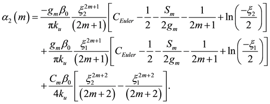
International Journal of Geosciences
Vol.05 No.13(2014), Article ID:52602,9 pages
10.4236/ijg.2014.513129
Determination of the Electromagnetic Field Created by Line Current and Sheet Current Source at the Earth’s Surface
Ghada M. Sami1,2, Maryam I. Al-Nami1
1Mathematics and Statistics Department, Faculty of Science, King Faisal University, Al-Hassa, KSA
2Mathematics Department, Faculty of Science, Ain Shams University, Cairo, Egypt
Email: g_sami2003@yahoo.com
Copyright © 2014 by authors and Scientific Research Publishing Inc.
This work is licensed under the Creative Commons Attribution International License (CC BY).
http://creativecommons.org/licenses/by/4.0/


Received 24 September 2014; revised 20 October 2014; accepted 15 November 2014
ABSTRACT
The electromagnetic field that generated by line current and sheet current at the surface of the earth can be expressed in analytical form. The line current created at the earth’s surface by an infinitely long line current is given by the inverse Fourier integrals over a horizontal wave number. The sheet current can be obtained by integrating the line current expansions using a Neumann and Struve functions; these functions have known mathematical properties, including the series expansions. The series expansions are exact with neglecting the displacement currents. Assuming a uniform earth and that there is no propagation, the three nonzero field components can be expressed in terms of the Neumann and Struve functions. The integrals of line current expansions are calculated by using the numerical methods. The results represented graphically and illustrated by figures. Results can be used to evaluate numerical solutions of more complicated modeling algorithms.
Keywords:
Electromagnetic Field, Transient Analysis, Series Expansions

1. Introduction
In the last few decades, there has been increased interest in the behavior of electromagnetic systems which are operated near a conducting earth. Many of these systems have been successfully used to measure the electromagnetic properties of the earth. That is, if the field of a transmitting source can be calculated in terms of idealized earth models, then measurements of actual fields near a real earth can be interpreted in terms of these models. This method is known as the induction method of geophysical exploration [1] [2] . A part of the integrand may be inverse Fourier integral form using the fast Fourier transforms such that the resulting integrals are known [3] . However, they presented only a particular form of decomposition of the integrand. Other studies have been applied to the probing of the fields in geological media [4] - [6] , determination of the current in a lightning return stroke [7] , the detection of nuclear bursts Johler [8] , and the discrimination of a radar scattered [9] . In the present study, we will focus on the effects caused by the presence of the earth’s surface. We are interested in the problem of electromagnetic field. Also, few electro-magnetic problems have been investigated along these lines [10] , [11] .
Electromagnetic boundary conditions at the surface of the wire were leading to a characteristic equation that determines the propagation constant along the wire [12] . Furthermore, Bishay et al. [13] computed the transient electromagnetic field of a vertical dipole on a two-layer conducting earth. Sami [14] calculated the influence of a magnetically permeable surface layer on transient electromagnetic field of a vertical magnetic dipole on a two- layer conducting earth. Bishay and Sami [15] studied Time-domain study of transient fields for a thin circular loop antenna. However, using a quasi-static approach, Wait [16] has derived closed-form solutions for the fields of loops above the surface of a two-layered earth, that are valid at sufficiently late times. A classical work in this subject is the remarkable book [17] and Wait [18] , for the electromagnetic fields of a phased line current over a conducting half-space. A very readable contemporary review was written by Olsen [19] who provides many significant references. Pirjola [20] considered the general case of a propagation current wave and derived formulas which give the electromagnetic field at the surface of the earth in an inverse Fourier integral form. The surface fields are also affected by currents induced within the ground and influenced by the conductivity of the Earth. This also has to be taken into account. Neglecting the currents displacement, thus making the quasi-static approximation, which is always permissible in geophysical applications, and assuming a uniform earth and that there is no propagation, the three nonzero field components can be expressed in terms of the Neumann and Struve functions. These functions have known mathematical properties, including their series expansions. The latter are utilized in this work to derive expressions for the electromagnetic field. In the previous work, the magnetic X and Z components are obtained from the electric Y component at the earth’s surface, neglecting the real part of electric field, and imaginary part of magnetic field.
The main objective of paper is to determine the electromagnetic field due to a line current and sheet current. Sheet current having a finite width implies a more realistic model. It can be obtained by integrating the line current expansions using a Neumann and Struve functions. These functions have known mathematical properties [21] , including the series expansions. The medium in which the line current lies in non-conducting (the air), and the other half-space is conducting (the earth). In this paper, the electric X and Z components are obtained from the magnetic Y component at the earth’s surface, we are considering the real and imaginary parts of electric field components and taking into account.
2. Line Current Model
In the Cartesian coordinate system (x, y, z), we assume that the earth’s surface is the xy plane, and the line current J flows is parallel to the y-axis at a height z = −d. The line current oscillating harmonically in time
 above a uniform half-space. The earth, characterized by a conductivity σ, a permittivity
 , a permeability μ, and a propagation constant K, where
 . (1)
. (1)
A model containing an infinitely long line current parallel to the surface between two half-spaces is frequently used in electromagnetic applications extending from geophysics. The medium in which the line current lies is nonconducting (the air), and the other half-space is conducting (the earth). The line current flows parallel to the y-axis at a height Z = ‒d. Neglecting displacement current effects, and assuming that
 is the vacuum permeability, then the propagation constant ᶄ of the earth is defined by
 . (2)
. (2)
The magnetic field has only the magnetic field component![]() , and the non-zero electric field components are
, and the non-zero electric field components are
![]() and
and![]() , now we shall give the expressions for the electromagnetic field as [22]
, now we shall give the expressions for the electromagnetic field as [22]
![]() , (3)
, (3)
![]() , (4)
, (4)
![]() . (5)
. (5)
R is the reflection coefficient at the earth’s surface is depending on the conductivity structure of the earth, and is given by,
![]() (6)
(6)
and J gives the magnitude of the line current oscillating harmonically in time![]() . To get the electric and magnetic fields at the earth's surface, then from Equations (3)-(5) we get,
. To get the electric and magnetic fields at the earth's surface, then from Equations (3)-(5) we get,
![]() (7)
(7)
![]() (8)
(8)
 (9)
(9)
The components of the electric fields are expressed in terms of
 through the relations
 , (10)
 . (11)
Equation (7) can be written in Terms of Struve function of the first order
 and the Neumann function of the first order
 [20] :
 (12)
(12)
The Neumann function
 and the Struve function
 can be expressed as a series expansion [20] ,
 , (13)
 , (14)
where
 denotes the Bessel function of the first order,
 is Eulers constant (≈0.5772) and
 is given by
 (15)
(15)
The function
 has the series expansion
 (16)
(16)
where
 is given by [21]
 . (17)
and
 is defined by
 . (18)
The gamma function Г satisfies,
 . (19)
The expansions of the Neumann and Struve functions Equation (13) and (14) with (16) may now be substituted into (12) to obtain a series representation for the magnetic field , which is straight forward algebra. It appears that the terms resulting from the function on the right-hand side of (13) exactly cancels the last term in (12), and the final series expansion can be written as
 , (20)
where
 , (21)
and
 , (22)
 . (23)
By applying the series expression of
 in (10) and (11) the series expansions of the components of the electric fields
 and
and
 are obtained in a straightforward manner as
 (24)
(24)
 .(25)
.(25)
3. Sheet Current Model
To determine the electromagnetic field created by the sheet current source at the surface, a sheet current can be lies in non-conducting (the air), and the other half-space is conducting (the earth). The sheet current having a finite width implies a more realistic model. It can be obtained by integrating the line current expansions using Neumann and Struve functions. We now consider an infinitely long sheet current on surface of the Earth. Let
 be the current distribution in the sheet. If the function
 can be normalized as follow,
 . (26)
Applying [(7)-(9)] for each line current
 lying at
 , the following formulas are obtained for the electric and magnetic fields at the Earth’s surface at a location determined by x can be written in the form
 , (27)
 , (28)
 . (29)
The electric field by (28) and (29) is expressible in terms of the magnetic field (28)
 , (30)
 . (31)
Rewriting (20) with
 and K replaced by
 and
and , this yields
 , (32)
where
 , (33)
and
 , (34)
 , (35)
where
 is the equivalent propagation constant and defined as
 , (36)
and if we assume that the wave number
 then the plane wave surface impedance can be written as
 . (37)
Let us define the functions
 and
and
 by
by
 , (38)
and
 . (39)
We know that
 , (40)
 (41)
(41)
 , (42)
and
 . (43)
A straightforward algebraic manipulation now allows for expressing (32) as
 , (44)
the quantities
 and
and
 given by
 , (45)
and
 (46)
(46)
where
 (47)
(47)
We now consider a uniform sheet located between
 and
and , then
 (48)
(48)
Assuming
 to be valid,
 , then the electric field components are obtained as:
 , (49)
 , (50)
where
 (51)
(51)
and
 (52)
(52)
 (a) (b) (c)
 (d) (e) (f)
 (g) (h) (i)
 (j) (k) (l)
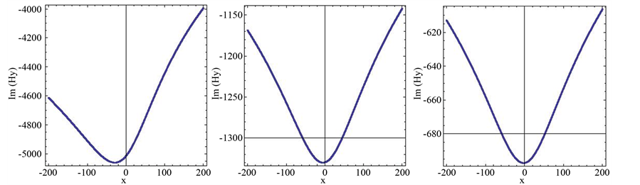
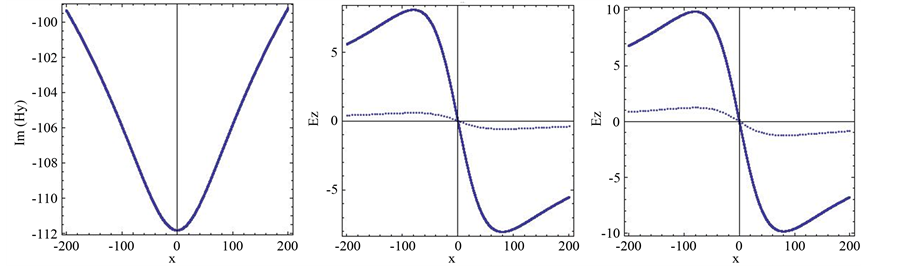
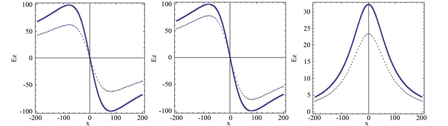
Figure 1.(a)-(d) represent the imaginary part of the magnetic field component Hy due to a line current of 1 MA with different values of distance x at the periods 10 s, 50 s, 100 s, and 700 s, respectively. (e)-(h) represent real and imaginary parts of the electric field component Ez, and (j)-(l) represent real and imaginary parts of the electric field component Ex, at the earth’s surface due to a line current of 1 MA with different values of x at the periods 10 s, 50 s, 100 s, and 700 s, respectively. The continuous and dots curves correspond to the real and imaginary part of the electric field, respectively.
![]() (a) (b) (c)
(a) (b) (c)
![]() (d) (e) (f)
(d) (e) (f)
![]() (g) (h) (i)
(g) (h) (i)
![]() (j) (k) (l)
(j) (k) (l)
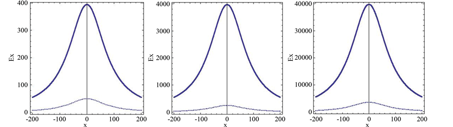
Figure 2.(a)-(d) represent the imaginary part of the magnetic field component Hy due to sheet current of 1 MA with different values of distance x at the periods 10 s, 50 s, 100 s, and 700 s, respectively. (e)-(h) represent real and imaginary parts of the electric field component component Ez, and (j)-(l) represent real and imaginary parts of the electric field component Ex, at the earth’s surface due to sheet current of 1 MA with different values of x at the periods 10 s, 50 s, 100 s, and 700 s, respectively. The continuous and dots curves correspond to the real and imaginary part of the electric field, respectively.
4. Numerical Results
Numerical computation of the electromagnetic field that generated by line current and sheet current at the surface of the earth can be easily performed, based on the Equations [(12), (24) and (25)] and [(44), (49) and (50)], respectively. The following parameters have been chosen to draw the curves shown by Figures 2(a)-(l):![]() ,
,
![]() ,
,![]() , and conductivity
, and conductivity![]() .
.
The electromagnetic field defined as a function of x coordinate at the surface of the earth due to line current and sheet current and plotted against the distance x.
For line current, Figures 1(a)-(d) represent the imaginary part of magnetic field component![]() , Figures 1(e)-(h) describe the real and imaginary part of electric field components
, Figures 1(e)-(h) describe the real and imaginary part of electric field components![]() , and
, and![]() , at the periods 10 s, 50 s, 100 s, and 700 s, respectively.
, at the periods 10 s, 50 s, 100 s, and 700 s, respectively.
For sheet current, Figures 2(a)-(d) represent the imaginary part of magnetic field component![]() , Figures 2(e)-(h) describe the real and imaginary part of electric field components
, Figures 2(e)-(h) describe the real and imaginary part of electric field components![]() , and
, and![]() , at the periods 10 s, 50 s, 100 s, and 700 s, respectively.
, at the periods 10 s, 50 s, 100 s, and 700 s, respectively.
The magnetic and electric fields were treated as complex quantities, the real part of the right-hand side of Equations (3)-(19) is ignored. It is seen that the magnetic field component
![]() is dominated by the imaginary part, and the real part of the electric field components
is dominated by the imaginary part, and the real part of the electric field components
![]() and
and
![]() are larger than the imaginary part.
are larger than the imaginary part.
The results we obtained that with increasing in the period indicate to increase in the imaginary part of magnetic field component![]() , and with increasing in period corresponding increasing in the values of the real and imaginary parts of the electric field components
, and with increasing in period corresponding increasing in the values of the real and imaginary parts of the electric field components
![]() and
and![]() .
.
We compared the magnetic and electric fields at the surface of a uniform earth with those produced by line current and sheet current.
In the sheet current, the values of the imaginary part of the magnetic field component
![]() are less than the values of the imaginary part of the magnetic field component
are less than the values of the imaginary part of the magnetic field component
![]() in the line current. The real and imaginary parts of the electric field component
in the line current. The real and imaginary parts of the electric field component
![]() in the sheet current are less than the electric field component
in the sheet current are less than the electric field component
![]() which obtained in the line current for the periods 10 s, 50 s, 100 s, and 700 s, respectively.
which obtained in the line current for the periods 10 s, 50 s, 100 s, and 700 s, respectively.
From a physical point of view, this means that the series expansions including the propagation constant
![]() is reasonable, the propagation constant
is reasonable, the propagation constant
![]() depends on the surface impedance. The absolute values of
depends on the surface impedance. The absolute values of
![]() and
and
![]() are less with
are less with![]() . While the sheet current of 1 MA parallel to the y-axis at height z = −d, the values of the real and imaginary parts of the electric field component
. While the sheet current of 1 MA parallel to the y-axis at height z = −d, the values of the real and imaginary parts of the electric field component![]() , is greater than the values of the real and imaginary parts of
, is greater than the values of the real and imaginary parts of
![]() in the line current, for the periods 10 s, 50 s, 100 s, and 700 s, respectively.
in the line current, for the periods 10 s, 50 s, 100 s, and 700 s, respectively.
5. Conclusions
We conclude that the electromagnetic field at the earth’s surface created by line current can be expressed in terms of the Neumann and Struve functions, and take the conductivity of the earth into consideration.
The magnetic and electric fields were derived in new series expansions and computations. Also we present the magnetic and electric fields due to sheet current obtained by integrating the line current expansion. The results are represented graphically. We compared the results of the magnetic and electric fields values at the surface of a uniform earth with those produced by line current with sheet current.
References
- Keller, G.V. and Frischknecht, F.C. (1966) Electrical Methods in Geophysical Prospecting. Pergamon Press, Oxford.
- Annan, A.P. (1973) Radio Interferometry Depth Sounding, Part I. “Theoretical discussion”. Geophysics, 38, 557-580. http://dx.doi.org/10.1190/1.1440360
- Tsang, L., Brown, R., Kong, J.A. and Simmons, G. (1974) Numerical Evaluation of Electromagnetic Fields Due to Dipole Antennas in the Presence of Stratified Media. Journal of Geophysical Research, 79, 2077-2080. http://dx.doi.org/10.1029/JB079i014p02077
- Wait, J.R. (1971) Electromagnetic Probing in Geophysics. Golem, Boulder, Colo.
- Bishay, S.T. and Sami, G.M. (2003) Natural-Frequency Concept Utilized in Remote Probing of the Earth. Canadian Journal of Physics, 81, 705-712. http://dx.doi.org/10.1139/p02-067
- Sami, G.M. (2005) Influence of a Magnetically Permeable Surface Layer on Transient Electromagnetic Field by Using Natural-Frequency Concept Utilized in Remote Probing of the Earth. Czechoslovak Journal of Physics, 55, 555-562. http://dx.doi.org/10.1007/s10582-005-0060-8
- Uman, M.A. and Mc Lain, D.K. (1970) Lightning Return Stroke Current from Magnetic and Radiation Field Measurements. Journal of Geophysical Research, 75, 5143-5147. http://dx.doi.org/10.1029/JC075i027p05143
- Johler, J.R. (1967) Propagation of Pulse from Nuclear Burst. IEEE Transactions on Antennas and Propagation, 15, 256-264. http://dx.doi.org/10.1109/TAP.1967.1138896
- Moffatt, D.L. and Mains, R.K. (1975) Detection and Discrimination of Radar Targets. IEEE Transactions on Antennas and Propagation, 23, 358-367. http://dx.doi.org/10.1109/TAP.1975.1141078
- De Hoop, A.T. and Frankena, H.J. (1960) Radiation of Pulses Generated by a Vertical Electric Dipole above a Plane Non-Conducting Earth. Applied Scientific Research, Section B, 8, 69-377.
- Langenberg, K.J. (1974) The Transient Response of a Dielectric Layer. Applied Physics, 3, 179-188. http://dx.doi.org/10.1007/BF00884494
- Wait, J.R. (1972) Theory of Wave Propagation Long a Thin Wire Parallel to an Interface. Radio Science, 7, 675-679. http://dx.doi.org/10.1029/RS007i006p00675
- Bishay, S.T., Abo-Seida, O.M. and Sami, G.M. (2001) Transient Electromagnetic Field of a Vertical Magnetic Dipole on a Two-Layer Conducting Earth. IEEE Transactions on Geoscience and Remote Sensing, 39, 894-897. http://dx.doi.org/10.1109/36.917919
- Sami, G.M. (2004) Influence of a Magnetically Permeable Surface Layer on Transient Electromagnetic Field of a Vertical Magnetic Dipole on a Two-Layer Conducting Earth. Czechoslovak Journal of Physics, 54, 339-348. http://dx.doi.org/10.1023/B:CJOP.0000018130.01468.df
- Bishay, S.T. and Sami, G.M. (2002) Time-Domain Study of Transient Fields for a Thin Circular Loop Antenna. Canadian Journal of Physics, 80, 995-1003. http://dx.doi.org/10.1139/p02-049
- Wait, J.R. (1972) On the Theory of Transient Electromagnetic Sounding over a Stratified Earth. Canadian Journal of Physics, 50, 1055-1061. http://dx.doi.org/10.1139/p72-146
- Sunde, E.D. (1968) Earth Conduction Effects in Transmission Systems. Dover Publications, New York.
- Wait, J.R. (1996) EM Fields of a Phased Line Current over a Conducting Half-Space. IEEE Transactions on Electromagnetic Compatibility, 38, 608-611. http://dx.doi.org/10.1109/15.544318
- Olsen, R.G. and Pankaskie, T.A. (1983) On the Exact, Carson and Image Theories for Wires at or above the Earth’s Interface. IEEE Transactions on Power Apparatus and Systems, PAS-102, 769-778. http://dx.doi.org/10.1109/TPAS.1983.317939
- Pirjola, R. (1982) Electromagnetic Induction in the Earth by a Plane Wave or by Fields of Line Current Harmonic in Time and Space. Geophysica, 18, 1-161.
- Arfken, G. (1985) Mathematical Methods for Physicists. 3rd Edition, Academic, San Diego, 985.
- I-Iermance, J.F. and Peltier, W.R. (1970) Magnetotelluric Fields of a Line Current. Journal of Geophysical Research, 75.