International Journal of Geosciences
Vol.4 No.7(2013), Article ID:36761,7 pages DOI:10.4236/ijg.2013.47096
Equivalent-Source from 3D Inversion Modeling for Magnetic Data Transformation
Applied Geophysics Research Group, Faculty of Mining and Petroleum Engineering, Bandung Institute of Technology, Bandung, Indonesia
Email: grandis@geoph.itb.ac.id, grandis@earthling.net
Copyright © 2013 Hendra Grandis. This is an open access article distributed under the Creative Commons Attribution License, which permits unrestricted use, distribution, and reproduction in any medium, provided the original work is properly cited.
Received July 1, 2013; revised August 3, 2013; accepted August 26, 2013
Keywords: Potential-Fields; Equivalent-Layer; Non-Uniqueness; Ambiguity; RTP; RTE; Upward Continuation
ABSTRACT
The well-known non-uniqueness in modeling of potential-field data results in an infinite number of models that fit the data almost equally. This non-uniqueness concept is exploited to devise a method to transform the magnetic data based on their equivalent-source. The unconstrained 3D magnetic inversion modeling is used to obtain the anomalous sources, i.e. 3D magnetization distribution in the subsurface. Although the 3D model fitting the data is not geologically feasible, it can serve as an equivalent-source. The transformations, which are commonly applied to magnetic data (reduction to the pole, reduction to the equator, upward and downward continuation), are the response of the equivalent-source with appropriate kernel functions. The application of the method to both synthetic and field data showed that the transformation of magnetic data using the 3D equivalent-source gave satisfactory results. The method is relatively more stable than the filtering technique, with respect to the noise present in the data.
1. Introduction
The concept of equivalent-source exploits the ambiguity or non-uniqueness in the modeling of potential-field (gravity and magnetic) data. When the response of an anomalous source is fit to the observed data, then we can calculate the response of such model with a different geometry, i.e. configuration of the observation positions relative to the anomalous sources. For example, the equivalent-source can be used to interpolate data at a homogeneous grid [1-3] or to obtain the field at a different height as in the upward or downward continuation transformation [4]. The reduction to the pole (or to the equator) of magnetic data can also be obtained from the equivalent-source with vertical (or horizontal) magnetization vector [5,6].
In general, the equivalent-source is represented by elementary sources, e.g. point mass for gravity or dipole for magnetic data, confined at a layer to conform with the potential field representation theory and to simplify the calculation. Therefore, in many literatures as in [2,3], the term equivalent-layer is also used for the equivalentsource. Mendonca and Silva [1] also introduced the concept of equivalent data for the use of only data that dominate the anomaly, while other data are considered as redundant and therefore can be ignored or discarded in the subsequent process.
The advances in computation performance and resources allow us to perform full 3D inversion modeling of gravity and magnetic data without any significant difficulty. The density or magnetization distribution of the equivalent-source can be extended to cover 3D space in the subsurface, rather than limited in a layer. This paper describes the application of 3D magnetic inversion to obtain 3D equivalent-source. The purely under-determined inversion with minimum-norm solution [7] may result in an unrealistic geological model of magnetization distribution. However, such model can be used as an equivalent-source for calculating transformations commonly applied to magnetic data. In this paper we focus on the reduction to the pole (RTP), reduction to the equator (RTE), and upward continuation of magnetic data. The application of the method to both synthetic and field data showed satisfactory results. The method is relatively more stable than the filtering technique, with respect to the noise present in the data.
2. Magnetic Inversion for 3D Model
The subsurface model for the anomalous sources is divided into elementary rectangular prisms with fixed dimension in x‑, y‑ and z‑axis. The magnetization of each prism is constant represented by m = [mj]; j = 1, 2,…, M with M is the number of prisms in the model. The magnetic anomaly d = [di]; i = 1, 2, …, N with N is the number of observation points, is given by,
 , (1)
, (1)
where G = [gij] is an N by M kernel matrix with gij being the magnetic anomaly at i-th observation point due to a unitary magnetization at the j-th prism. The magnetic response of an elementary prism gij is calculated by using the well-known formula implemented by Blakely [8] in the subroutine mbox.
Equation (1) represents a linear relationship between the subsurface magnetization distribution (or model m) and the magnetic anomaly (or data d). It allows the calculation of the theoretical magnetic data for a known magnetization model, i.e. the 3D magnetic forward modeling. The inverse problem to estimate the model from the data is linear. However, since the observation points are located only at the earth’s surface, the number of the data (N) is certainly much less than the number of the model parameters (M). The number of model parameters M is a multiplication of the number of prisms along x‑, y‑ and z‑axis (Figure 1).
For such under-determined inverse problem [7], the standard minimum-norm solution is expressed by,
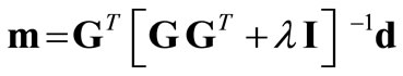 , (2)
, (2)
where λ is the damping factor, I is a unitary matrix and the super-script T denotes the matrix transposition. The damping factor is used to avoid over-fitting, i.e. unnecessary detail of the model reproducing noise in the data. The choice of λ is usually determined by trial-and-error.
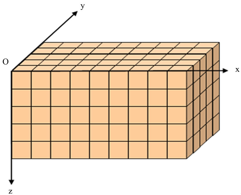
Figure 1. Discretization of the subsurface into a number of rectangular prisms in x‑, y‑ and z‑axis for 3D magnetic modeling.
However, to minimize the ad hoc manner in the choice of λ, Mendonca and Silva [1,2] used a normalization matrix D such that λ can be chosen in the interval [0,1]. The N by N diagonal normalization matrix D is given by,
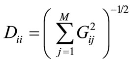 . (3)
. (3)
Then, Equation (2) becomes,
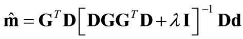 . (4)
. (4)
The inversion of matrix in Equation (2) or its modified or normalized version shown in Equation (4) involves a large matrix that may become unstable. To stabilize the inversion, the Singular Value Decomposition (SVD) technique is usually employed [7,9]. In the application of the SVD technique, singular values less than a threshold value are considered as negligible and set to zero such that they are discarded from the solution calculation. In the cases described in this paper, singular values less than 10−6 times the maximum singular value are neglected which result in satisfactory solutions.
Equation (2) or (4) represents the solution of the unconstrained 3D magnetic inversion, except that model norm is minimized. The inverse model tends to be concentrated near the earth’s surface due to the ambiguity or non-uniqueness problem inherent in the modeling of potential-field data. This mathematical solution provides little information about the true structure of the subsurface. Nevertheless, such model can still be exploited as the 3D equivalent-source for transformation of magnetic data.
3. Magnetic Data Transformation
In geophysical prospecting using magnetic method, we conventionally consider that all anomalies are the results of the earth’s permanent magnetic field induction into the rocks containing magnetic minerals. Therefore, the magnetic anomalies are influenced by the inclination of the inducing field. The observed anomaly generally has dipolar character, i.e. negative and positive closed contours. This dipolar signatures lead to difficult qualitative interpretation of the magnetic data. The anomaly may not be directly located above the causative sources.
The reduction to the pole (RTP) transformation is intended to obtain magnetic anomaly as if the inducing field is vertically downward, i.e. at the north pole. For the survey area at low magnetic latitude, it is considered more appropriate to perform the reduction to the equator (RTE). Both transformations will render the anomaly more or less monopolar, thus facilitate the qualitative interpretation [8]. The upward continuation is aimed at bringing the observation points as if they are above the actual measurement points. This will result in smoother anomalies due to increasing distance between the observation points to the causative sources. This transformation is usually performed to obtain the regional component of the anomalies. All magnetic data transformations are generally performed by using the filtering technique in the spatial frequency domain [8] following the general formula,
 , (5)
, (5)
where T and TX are the input and output of the transformation process respectively, ΨX is the filter transformation function and F[∙] represents the 2D Fast Fourier Transform (FFT).
Equation (5) states that in the Fourier domain the transformed (RTP, RTE or upward continued) magnetic data can be obtained from the multiplication of the data with the appropriate filter function. The transformed magnetic data (in spatial domain) are the inverse FFT or F[∙]−1 of the result of Equation (5). The application of the filtering technique to transform magnetic data usually enhances high frequency components of the data. Therefore, the transformed results usually appear more noisy. In addition, the RTP transformation is generally unstable for magnetic data from low latitude regions, although we have the RTE as an alternative. This is due to the RTP filter function containing a factor inversely proportional to the inclination, while inclination at low latitude (near magnetic equator) is very small [6,10].
Equation (1) also states that the data are the response of the subsurface magnetization model with the kernel matrix G. This kernel matrix retains information on the relative geometry of the source and the observation points and also the direction of the inducing field. The transformed magnetic data can simply be viewed as the response of the 3D equivalent-source obtained from Equation (4) with the appropriate kernel matrix,
 . (6)
. (6)
where d*, G* are transformed magnetic data and the associated kernel matrix respectively. For the reduction to the pole (or to equator), the magnetic inducing field direction would be vertical (or horizontal). For the upward continuation, the geometry of the observation points would be at a certain height above the actual measurement points. With this method, the magnetic data usually at the uneven topographic surface do not need to be levelled to the same height before the upward continuation [11].
4. Results and Discussion
4.1. Synthetic Data
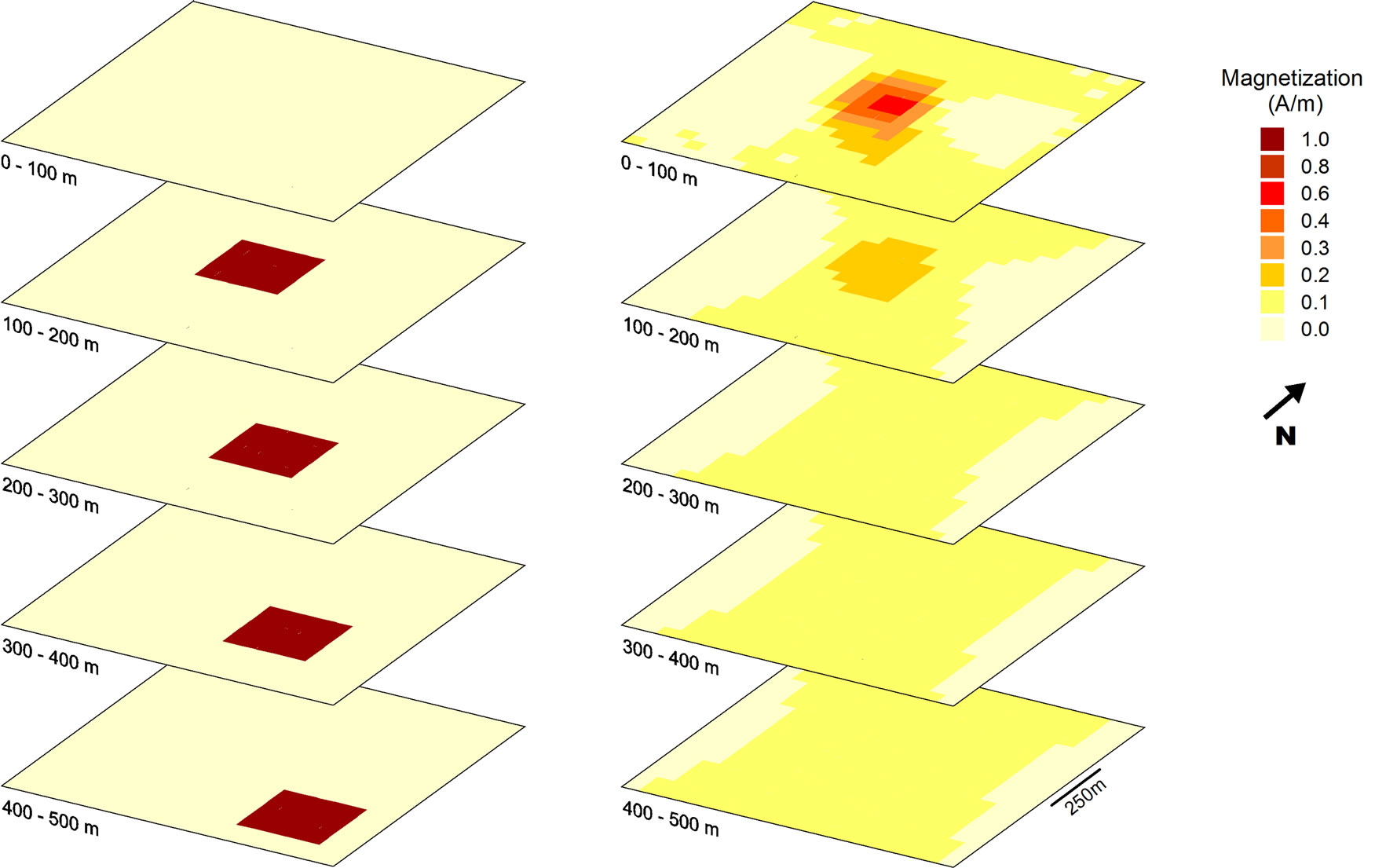
A synthetic model was constructed by discretizing the subsurface into 20 by 20 by 10 prisms along x, y and z directions with each prism measures 50 by 50 by 50 meters in dimension. The anomalous magnetized body consists of blocks with 250 by 250 meters in horizontal dimension placed from 100 to 500 meters depth (see Figure 2(a)). The magnetization of the anomalous body is 1.0 Ampere/meter with the inclination and declination are –10˚ and 0˚ respectively, simulating an anomaly at the southern magnetic low latitude. The gaussian noise with zero mean and 2 nanoTesla standard deviation were added to the synthetic data.
The result of uncontrained inversion using l = 0.1 is shown in Figure 2(b). As expected, the inverse model did not recover the synthetic model at all. The anomalous source tends to be concentrated near the surface with the magnetization much less than 1.0 Ampere/meter [12]. The depth of the anomaly represented by such inverse model is certainly erroneous. However, the recovered model represents the data consistently as can be seen in Figure 3 comparing the synthetic data and the response of the inverse model. In Figure 3, the interval contour is set to 2 nanoTesla to enhance the details on both magnetic anomaly maps. The anomalous source from the inversion is shallow with lower magnetization intensity. This results in a narrow and low magnitude magnetic anomaly, especially for the dominant lower magnitude (negative values), compared to the synthetic data.
The obtained 3D equivalent-source was then used in the transformation of the synthetic magnetic data for the reduction to the pole, reduction to the equator and upward continuation by applying Equation (6). We also performed the transformation of the same synthetic data using the filtering technique in the frequency domain. In applying Equation (5), the 2D FFT subroutines fourn and newvec from Blakey [8] was used.
The results of transformation using the 3D equivalentsource and also the filtering technique in the frequency domain are presented in Figure 4. In general, the transformations using the 3D equivalent-source show relatively better results, judging from the expected pattern of the anomaly. In addition, the transformation using the 3D equivalent-source is also more robust, i.e. less influenced by the noise present in the data. The RTP using the filtering technique exhibits dominant linear artefacts in the North-South direction (Figure 4(a), right panel). These might be related to the low latitude effect of the data [6,10]. The FFT technique is also sensitive to edge effects such that it has to be applied cautiously.
4.2. Field Data
The magnetic field data are from a private concession for artisanal gold mining operated by a local community in the southern part of West Java province, Indonesia. The objective of the survey was to delineate the magnetized anomalous source usually associated with intrusive dike. As the by-product of the intrusion, the mineralization that
 (a) (b)
Figure 2. Synthetic model (a) and inverse model (b). The models are shown only every 100 meters interval for simplicity.

Figure 3. Comparison of the synthetic data (left) and the calculated response of the inverse model (right). The interval contour is 2 nanoTesla to enhance the details on both magnetic anomaly maps.
occurs in quartz veins may contain gold as ore, although usually very small in quantity. The survey area measuring only 1000 by 600 meters was covered by North to South traverse lines with 100 meters distance between the lines. The station spacing on the lines was 12.5 meters. The data and results presented in this paper are focused on an area of 600 by 600 meters.
The magnetic data were corrected for IGRF values that include a constant regional component, since the area is very small. The inclination and declination are –34˚ and 0˚ respectively. Figure 5 shows the field data along with the response of the inverse model. The 3D equivalent-
 (a)
(a) (b)
(b)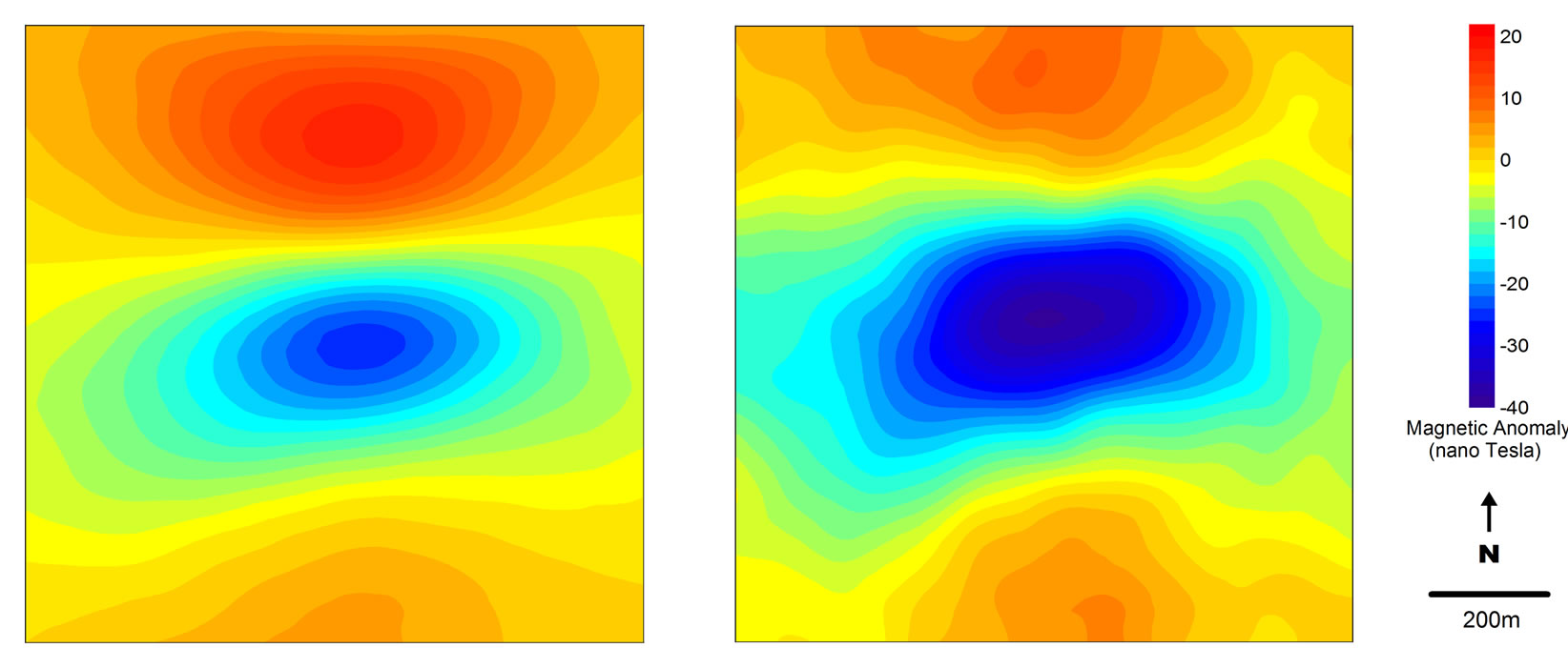 (c)
(c)
Figure 4. Comparison of the magnetic data transformation using the 3D equivalent-source (left) and the filtering technique in the Fourier domain (right), for reduction to the pole (a), reduction to the equator (b) and 50 meters upward continuation (c).
source is not shown as it does not represent the actual subsurface structure. The contour interval and colour scale are the same for both maps for direct comparison. The equivalent-source response has lower amplitude compared to the field data. The discrepancies in the details are obvious especially at the South-Eastern part of the area. In this case, the 3D equivalent-source was obtained by using a damping factor of 0.4 such that the inverse model did not replicate the noise.
The RTP and RTE transformations of the field data are presented in Figure 6. The anomalies in the RTP and RTE maps are usually in opposite magnitude, low in one map becomes high in the other map and vice versa. The interesting anomaly associated with a magnetized body crosses almost diagonally the survey area (marked by white dashed lines). This anomaly is represented by high magnetic anomaly in the RTP map or low anomaly in the RTE map. We assume that anomalies near the border of the maps may contain a certain degree of edge effects.
Therefore, we do not consider those anomalies. Other anomalies, especially at the South and South-Eastern part of the map, are also doubtful and assumed to be insignificant. These dubious anomalies coincide with the discrepancies observed between the field data and the response of 3D equivalent-source (see Figure 5).
The anomaly delineated from the RTP and RTE maps is well correlated with the quartz vein observed at the shallow part of the subsurface. This quartz vein is possibly the effect of an intrusive dike. Further analysis using the modeling with depth resolution capability [13] may result in more quantitative information on the subsurface extent and geometry of this anomaly.
5. Conclusions
The unconstrained 3D magnetic inversion results in a model that can be used as an equivalent-source. The utility and validity of the 3D equivalent-source for

Figure 5. Magnetic anomaly maps of the field data (left) and the theoretical response of the inverse model or the 3D equivalent-layer (right).

Figure 6. Magnetic anomalies reduced to the pole (left) and reduced to the equator (right) of the field data. The white dashed lines delineate the interesting anomaly that might be associated with subsurface intrusive dike.
magnetic data transformation, i.e. reduction to the pole, reduction to the equator and upward continuation, have been demonstrated with synthetic and field data. The method proposed in this paper is also relatively robust to the presence of noise in the data. However, the process to invert the magnetic data to obtain the 3D equivalentsource may take longer execution time than the conventional magnetic data transformation using the filtering method. This will not impose any difficulty using the current computation technology and resources.
The 3D equivalent-source can be extended to gravity data as both gravity and magnetic methods exhibit nonuniqueness and ambiguity in their modeling. Similarly to other equivalent-source approaches, the present method can also serve as data interpolation, gridding and smoothing method. The use of potential-field gradient data, especially full gravity gradient tensor for prospect scale detailing is currently increasing, e.g. [14,15]. In general, to simulate the gradient tensor from the single vertical component data, the FFT technique is also employed [16]. In this perspective, the 3D equivalent-source may also serve as an alternative to the evaluation of the gradient tensor both for magnetic and gravity.
The upward continuation using 3D equivalent-source can be used to support the potential-field modeling with depth resolution as poposed for example by Fedi and Rapolla [13]. However, the use of potential-field data at several heights is still debatable, e.g. [17]. Data at different levels, especially as a result of the upward continuation, are considered to have no additional information on the vertical distribution of the anomalous sources. Nevertheless, data at different heights may contain information on the gradient and curvature of the field from which an insight about the decaying rate related to the distance (i.e. depth) may be inferred. We are still investigating such possibility in our ongoing research.
REFERENCES
- C. A. Mendonca and J. B. C. Silva, “The Equivalent Data Concept Applied to the Interpolation of Potential Field Data,” Geophysics, Vol. 59, No. 5, 1994, pp. 722-732. doi:10.1190/1.1443630
- C. A. Mendonca and J. B. C. Silva, “Interpolation of Potential-Field Data by Equivalent Layer and Minimum Curvature: A Comparative Analysis,” Geophysics, Vol. 60, No. 2, 1995, pp. 399-407. doi:10.1190/1.1443776
- G. R. J. Cooper, “Gridding Gravity Data Using an Equivalent Layer,” Computer and Geosciences, Vol. 26, No. 2, 2000, pp. 227-233. doi:10.1016/S0098-3004(99)00089-8
- L. Cordell, “A Scattered Equivalent-Source Method for Interpolation and Gridding of Potential-Field Data in Three Dimensions,” Geophysics, Vol. 57, No. 4, 1992, pp. 629-636. doi:10.1190/1.1443275
- D. A. Emilia, “Equivalent Sources Used as an Analytic Base for Processing Total Magnetic Field Profiles,” Geophysics, Vol. 38, No. 2, 1973, pp. 339-348. doi:10.1190/1.1440344
- J. B. C. Silva, “Reduction to the Pole as an Inverse Problem and Its Application to Low-Latitude Anomalies,” Geophysics, Vol. 51, No. 2, 1986, pp. 369-382. doi:10.1190/1.1442096
- W. Menke, “Geophysical Data Analysis: Discrete Inverse Theory,” 3rd Edition, Academic Press, London, 2012.
- R. J. Blakely, “Potential Theory in Gravity and Magnetic Applications,” Cambridge University Press, Cambridge, 1995. doi:10.1017/CBO9780511549816
- W. H. Press, B. P. Flannery, S. A. Teukolsky and W. T. Vetterling, “Numerical Recipes: The Art of Scientific Computing,” 2nd Edition, Cambridge University Press, Cambridge, 1997.
- K. I. Kis, “Transfer Properties of the Reduction of Magnetic Anomalies to the Pole and to the Equator,” Geophysics, Vol. 55, No. 9, 1990, pp. 1141-1147. doi:10.1190/1.1442930
- S.-Z. Xu, C.-H. Yang, S. Dai and D. Zhang, “A New Method for Continuation of 3D Potential Fields to a Horizontal Plane,” Geophysics, Vol. 68, No. 6, 2003, pp. 1917-1921. doi:10.1190/1.1635045
- Y. Li and D. W. Oldenburg, “3-D Inversion of Magnetic Data,” Geophysics, Vol. 61, No. 2, 1996, pp. 394-408. doi:10.1190/1.1443968
- M. Fedi and A. Rapolla, “3-D Inversion of Gravity and Magnetic Data with Depth Resolution,” Geophysics, Vol. 64, No. 2, 1999, pp. 452-460. doi:10.1190/1.1444550
- A. H. Saad, “Understanding Gravity Gradients—A Tutorial,” Leading Edge, Vol. 25, No. 8, 2006, pp. 942-949. doi:10.1190/1.2335167
- G. Barnes, “Interpolating the Gravity Field Using Full Tensor Gradient Measurements,” First Break, Vol. 97, No. 4, 2012, pp. 97-101.
- K. L. Mickus and J. H. Hinojosa, “The Complete Gravity Gradient Tensor Derived From The Vertical Component of Gravity: A Fourier Transform Technique,” Journal of Applied Geophysics, Vol. 46, No. 3, 2001, pp. 156-176. doi:10.1016/S0926-9851(01)00031-3
- D. W. Oldenburg and Y. Li, “On ‘3-D Inversion of Gravity and Magnetic Data with Depth Resolution’ (M. Fedi and A. Rapolla, Geophysics, 64, 452-460),” Geophysics, Vol. 68, No. 1, 2003, pp. 400-402. doi:10.1190/1.1552007