International Journal of Geosciences
Vol.4 No.6(2013), Article ID:35848,19 pages DOI:10.4236/ijg.2013.46089
Past, Present and Future Climate of Antarctica
Earth System Science Organization, National Centre for Antarctic and Ocean Research, Ministry of Earth Sciences, Goa, India
Email: alvluis1@gmail.com
Copyright © 2013 Alvarinho J. Luis. This is an open access article distributed under the Creative Commons Attribution License, which permits unrestricted use, distribution, and reproduction in any medium, provided the original work is properly cited.
Received May 27, 2013; revised June 29, 2013; accepted July 6, 2013
Keywords: Component Antarctic Climate; Discovery; Sea Ice; Glaciers; Southern Hemisphere Annular Mode; Antarctic Warming
ABSTRACT
Anthropogenic warming of near-surface atmosphere in the last 50 years is dominant over the west Antarctic Peninsula. Ozone depletion has led to partly cooling of the stratosphere. The positive polarity of the Southern Hemisphere Annular Mode (SAM) index and its enhancement over the past 50 years have intensified the westerlies over the Southern Ocean, and induced warming of Antarctic Peninsula. Dictated by local ocean-atmosphere processes and remote forcing, the Antarctic sea ice extent is increasing, contrary to climate model predictions for the 21st century, and this increase has strong regional and seasonal signatures. Models incorporating doubling of present day CO2 predict warming of the Antarctic sea ice zone, a reduction in sea ice cover, and warming of the Antarctic Plateau, accompanied by increased snowfall.
1. Introduction
Antarctica was discovered by James Cook who crossed the Antarctic Circle and circumnavigated the continent in 1773. The first landing on the continent was accomplished by the Norwegian whaling ship Antarctic in 1895, while the British were the first to spend a winter on Antarctica in 1899. The first recorded settlement on Antarctica is the Orcadas station (60˚44.25'S, 44˚44.33'W) that was set up on Laurie Island in 1903. In 1957, the International Geophysical Year provided a fillip to the Antarctic expeditions which led to the establishment of permanently manned stations at many points around the continent. Airplanes first landed on Antarctica when Australian Hubert Wilkins flew 2092 km over the Antarctic Peninsula in the 1920s. Richard Byrd took the first Antarctic flight in 1929 and discovered a new mountain range which he named Rockefeller. Byrd continued the Antarctic explorations for three decades and revolutionized the use of modern vehicles and communications equipment for polar exploration. Though Antarctica still remains an enigma, from the point of being isolated, mysterious and inhospitable, there is, however, greater accessibility by air via the ice runways and by sea which is being offered by different countries through their science programmes and adventure tourism.
Antarctica is the coldest, windiest, and driest continent with a repository of more than 70% of the Earth’s freshwater in the form of ice sheet. Despite its thick ice sheet, very little moisture falls from the sky over Antarctica. The inner regions of the continent receive an average precipitation of 51 mm/yr, primarily in the form of snow, while the coastal regions receive only average 203 mm per year. The mean precipitation minus evaporation for the 20th century for the whole continent is in the range of 150 - 190 mm/yr [1]. The threatening experiences in Antarctica are wind chill and blizzard which is a combination of gale force winds (~160 km/h), blowing snow and poor visibility. It is the highest continent with numerous mountain ranges with an average height of 2500 m. With a length of 3500 km and a width of 100 - 300 km, the Transantarctic Mountains forms the longest boundary between East and West Antarctica (Figure 1). With a large change in the altitude from coast to the Antarctic Plateau, cold and dense pool of air flows out from the polar plateau. As the wind descends the steep vertical cliffs with heaps of snow, it is accelerated by gravity and spreads out towards the coast forming katabatic winds.
Antarctica hosts numerous fresh water and saline lakes in the ice-free oases on the edge of the continent such as the Vestfold Hills, Larsemann Hills and McMurdo Dry Valleys, which colonized by various organisms. The size of the lakes ranges from small ponds to an area greater than 10 km2, in depth from a few centimeters to over 300 m, and in age from a single summer to several full glacial cycles. Those that contain liquid water throughout the year, with either seasonal or perennial ice insulating the water against heat loss and complete freezing, are generally referred to as lakes while those that freeze to the base during winter (typically <2 m deep) are referred to as ponds. Most of these lakes postdate the Last Glacial Maximum, between 25,000 and 18,000 years ago, when the ice sheet expanded over many of the coastal oases and across the continental shelf. Epiglacial lakes are the most common lakes in Antarctica, which are usually formed in depressions at the boundary between areas of rock and ice and are often perennially ice-covered. Supraglacial lakes are found on the surface of the ice sheet, glaciers, and ice shelves, which range from cryoconite holes, less than a meter across, to melt water lakes that can extend to several square kilometers. Chemically, the lakes contain fresh to hypersaline water with concentrations of salt exceeding eight times that of seawater, which prevents them from freezing during winter when their water column temperature drops below −10˚C. Many saline lakes exhibit seasonal or permanent stratification of their water columns due to temperature and salinity gradients.
The continent is surrounded by sea ice which range from about two million square kilometers in January/ February (austral summer) to thirteen million square kilometers in September/October (austral winter). Since the reliable satellite-based monitoring started in 1979, Antarctic sea ice extent (the total area covered by at least 15% of ice) shows slight increasing trend of 0.6% ± 0.5% per decade (http://nsidc.org/data/seaice_index). However, this small Antarctic sea ice increase is actually the result of much larger regional increases and decreases, which are caused by wind-driven changes [2]. In some regions, enhanced northward winds cause the sea ice to spread outwards from the continent. The sea ice extent peaked at 19.44 million km2 on 26 September 2012. All the activities on this land are governed by Antarctic treaty which came into force in 1961 with twelve original signatories. Under this treaty Antarctica is the land that symbolizes unity and fraternity—a land of no war, no conflict, no mining, a land of solidarity, and a land of scientific research. To date, the Antarctic Treaty has 48 member countries, a number of observer countries, and several non-governmental organizations.
2. Antarctic Evolution and Climatic Events
Antarctica, as it appears today exists for the past 60 million years, but it has not always been located where it is now, nor has it always been so cold. Antarctic history dates back to giant Southern Hemisphere land-mass known as Gondwanaland, which existed from 500 to 160 million years ago. At this time the eastern part of Antarctica formed the core of this super continent which also included Africa, South America, India, Australia and New Zealand. Evidence for this link up can be found in the similar geological features of the southern parts of these continents, which led Alfred Wegner to propose his theory of Continental Drift in 1912 [3] that set the foundation to the development of theory of plate tectonics. It suggests that the continents move about on convection currents in the earth’s molten interior. The supercontinent began splitting about 183 million years ago, during the Jurassic period. The violent volcanic eruptions swept past the land and ocean beds and caused extinction of many species including dinosaurs. Indian plate separated from that of Antarctic about 100 million years ago, Australia about 40 million years ago and South America was the last to separate at around 23 million years before present. This opened the sea route—the Drake Passage—between South America and Antarctica about 28 million years from present, isolating the latter from the warmer world and ushering the formation of ice sheet on Antarctica.
Antarctic continent is divided into East Antarctica and West Antarctica, which are quite different geologically from each other (Figure 1). East Antarctica consists of a stable shield of pre-Cambrian rocks older than 570 million years and mostly above sea-level. West Antarctica would be simply a string of islands, if the ice cover were removed. The two regions are separated by the TransAntarctic Mountains extending from the tip of the Antarctic Peninsula to Cape Adare, spanning a distance of about 3500 km. East Antarctica is colder than its western counterpart. In most places, about 2% - 4% of the area are exposed which consists of isolated tips of mountains (nunataks), the edges of the continent where the ice sheet leaves exposed rock and oases that have been exposed both through postglacial retreat of the ice cap and isostatic rebound of the Earth’s crust following the most recent deglaciation. The largest oases are found near the coast of the Ross Sea, and are known as the McMurdo Dry Valleys. Other large oases are found in eastern Antarctica including the Vestfold Hills, Larsemann Hills, Bunger Hills, Schirmacher Oasis, Syowa Oasis, and on the Antarctic Peninsula at Ablation Point on the east coast of Alexander Island. The coast of Antarctica is more densely populated with ice shelves, and nearly half the coastline consists of floating ice.
The present climate over the Antarctica is a result of interaction of the cryosphere-ocean-atmosphere and can be briefly summarized as follows. With a decline in CO2 level and air temperature at above 4˚C than the present [4,5], ice sheets were formed around 34 Ma ago [6]. The ice sheets spanned all over the Antarctic continent,
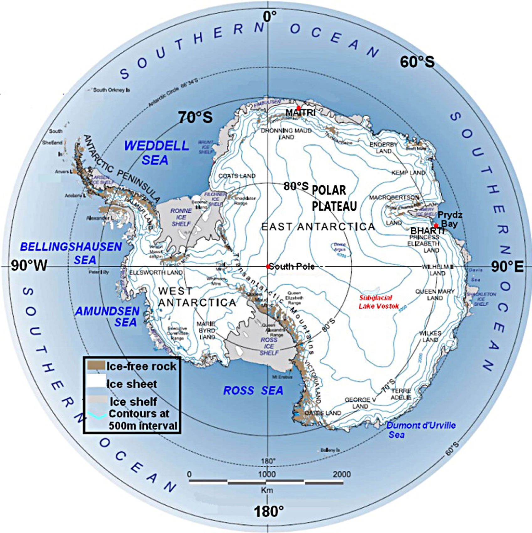
Figure 1. Land topography and geographical locations of key places and regions in Antarctica.
although they were warmer and thinner than present. With a gradual decrease in global CO2 levels, thick ice sheets covered Antarctica about 14 Ma ago [7]. Ice core records from East Antarctica reveal an early Holocene climatic optimum from 11.5 to 9 ka ago, followed by a cold event about 8 ka ago, then a return to mid-Holocene warm conditions, and followed by a slow cooling that ended with the rise in CO2 post-1850. Overlapping on these long-term trends are millennial scale oscillations, some of which involves relatively abrupt events that saw strengthening of the westerlies and development of a massive Amundsen Sea Low in the South Pacific, accompanied by cooling over East Antarctica, between 6000 and 5000 AD and other between 1700 and 1000 AD.
3. Antarctic Atmospheric Chemistry
The Antarctic air, snow, and ice bears the testimony of anthropogenic chemicals which have accumulated over time scales ranging from storm events to hundreds of thousands of years. Over Antarctica springtime depletion of stratospheric ozone 10% below normal of January levels was detected in 1984, by using measurements from ground-based Dobson spectrophotometers [8] over Halley Bay, Antarctica. A long-term trend derived from satellite observations and ground-based measurements (ozonesonde, Brewer spectrophotometer, etc.) suggest that the ozone hole grew rapidly in size and depth from 1980 to 2000 (Figure 2(a)) because global emission of ozonedepleting substance like chlorofluorocarbons (CFC) from several industrial processes peaked at 2.1 million tonnes per year, and by 2005 it declined by 70% to 0.5 million tones.
The ozone, which forms a protective layer at about 15 - 10 km altitude, is catalytically depleted by reactive chlorine gases which release ClOx radicals on the surface of ice crystals in polar stratospheric clouds [9]. These radicals are set free by the industrial compounds—the CFCs. The destruction takes place in the austral spring (August - October), when the sun begins to rise, heating the stratosphere and supplying UV rays that convert chlorine gas to the chlorine atoms that attack ozone molecules. This chemical reaction is facilitated because the Antarctic stratosphere cools down to below −78˚C. That coldness is sustained by strong stratospheric winds that blow clockwise around the continent during austral winter to form a wall of moving air called the polar vortex.

Figure 2. Annual-mean time series of ozone hole area and column ozone observed by Total Ozone Mapping Spectrometer (1978-2005) and Ozone Monitoring Instrument (OMI) (2005 onwards) processed with the Version 8 algorithm that has been developed by NASA Goddard’s Ozone Processing Team.
Inside the vortex the temperatures drops as the supply of warm air from outside is terminated, causing the water vapor to condense into tiny ice particles leading to the formation of polar stratospheric clouds. These clouds draw the chlorine-bearing compounds that are released by industrially produced CFCs. Man-made CFCs enter the stratosphere primarily from the tropical upper troposphere and accumulates in the stratosphere; the air motions then transport these gases upward and toward the pole in both hemispheres.
By October, the solar radiation warms up the air, melting the icy particles that make up the polar stratospheric clouds and the ozone destruction stops. The molecules that were bound to their icy surfaces are released to bind chlorine gas, arresting its breakdown into destructive chlorine atoms. By November, the polar vortex disintegrates, facilitating the flow of ozone rich air from outside thereby, replenishing the ozone that was destroyed. The ozone levels in the stratosphere are restored back to normal, until the following spring when the process begins again. A reduction in the emissions of ozone-depleting substances [10] has diminished the ozone hole (Figure 2(a)) by about 60%. Its intensity however varies from year to year depending on variability in atmospheric conditions. For example, in the austral spring of 2002, a sudden stratospheric warming caused a significant reduction in the size of the ozone hole, leading to higher ozone concentrations than usual. Observation from 1985 to 2002 have revealed that the lower part of the stratosphere has cooled by 10˚C, as a result the time of decay of the polar vortex has shifted from early November during the 1970s to late December in the 1990s [11]. It is inferred that a cooler stratosphere may in turn strengthen polar stratospheric cloud formation thereby, aggravating the conditions for ozone depletion. This inversion type of scenario could enhance further warming of the Antarctic troposphere.
A call to phase down the global production, consumption and emissions of ozone-depleting substances (OSDs) was made at the Montreal Protocol, which was negotiated and signed by 24 countries and by the European Economic Community in September 1987 [12]. Under the Montreal Protocol and national regulations, significant decreases have occurred in the production, use, emissions, and observed atmospheric concentrations of CFC- 11, CFC-113, methyl chloroform, and several other ODSs [10] and there is emerging evidence for recovery of stratospheric ozone [13]. Further progress was made at the Kyoto Protocol wherein the United Nations Framework Convention on Climate Change [14] set binding obligations on the industrialized countries to reduce their emissions of greenhouse gases (CO2, CH4, N2O, HFCs, PFCs, and SF6) in the atmosphere to 1990 baseline in order to prevent dangerous anthropogenic interference with the climate system. The Protocol was initially adopted on 11 December, 1997 in Kyoto and entered into force on 16 February, 2005. As of September 2011, 37 developed nations have signed and ratified the protocol, except for USA which did not ratify the same. The pollution-reduction commitments made by industrialized nations expired on 31 December 2012.
Chemicals like Pb have entered Antarctica as early as 1880s [15] through the use of leaded gasoline in vehicles engaged for logistic operations. Eolian fallout flux of lead in Antarctica is estimated to be about 0.07 ng Pb/ cm2/yr, while snow cores covering the last two centuries collected at an inland site in East Antarctica showed concentration of 1.7 pg∙Pb/g [16]. Over the decades, the Pb concentration has increased 2 to 3 folds as a result of industrial lead pollution; however, a decreasing trend in Pb levels is observed during recent years with the phasing out of Pb additives in gasoline. Low concentrations of trace metals such as Cr, Cu, Zn, Ag, Pb, Bi, and U, have been detected as a consequence of aerial transport from surrounding continents [17-21]. In the last 50 years, increases in anthropogenic source pollutants, including trace elements, is partly due to Antarctic logistic activeties and the industrial activity in the Northern Hemisphere. POPs such as polychlorobiphenyls and chlorineated pesticides such as DDT and hexachloribenzene are also detected in the Antarctic environment [22-25]. Radionuclides released from above-ground nuclear explosions and also from Chernobyl nuclear accident have been detected [26] throughout Antarctica.
Though sea spray dominantly contributes to the ionic budget of the atmospheric aerosol on global scale, formation of fragile structures of sea-salt crystals, known as frost flowers, caused by evaporation/condensation seawater processes during sea-ice growth is the source of sea-salt components (ssNa+, ssMg2+ and ssCl−) to polar atmosphere [27,28]. ssNa+ is the dominant fraction of the Na+ budget, contributing more than 80% of the sea-spray components. The concentration of ssNa+ varies from ~2 to ~30 ppb in the East Antarctic and from ~75 to ~15,000 ppb at coastal sites [29]. Higher values close to the coast are attributed to the influence of either cyclones (ssNa+ rich) or katabatic winds (ssNa+ depleted). ssCl− from marine source exhibits a range from ~1 to ~28,000 ppb, with highest values at coastal sites (~150 to ~28,000 ppb) and lower values in the interior (1 to ~150 ppb) [29]. The Antarctic Peninsula shows overall high values of ssNa+ and ssCl−. The spatial variability of multisource (biomass, lightning, marine, and human activity)  ranges from ~4 to ~800 ppb; highest concentration is detected in Enderby Land, Dronning Maud Land, and Victoria Land (~30 to 800 ppb) [29]. The lowest values for
  are observed at the Antarctic Peninsula and Kaiser Wilhelm II Land. The spatial variability
  sourced from biomass, lightning, marine, and human activity ranges from ~4 to ~800 ppb. Highest values are observed in Enderby Land, Dronning Maud Land, and Victoria Land, ranging from ~30 to 800 ppb, while lowest values are observed at the Antarctic Peninsula and Kaiser Wilhelm II Land [29]. The spatial variability of
![]() , which is produced from marine, evaporite, volcanic, and human activity, ranges from 0.1 to ~4000 ppb. The source for
, which is produced from marine, evaporite, volcanic, and human activity, ranges from 0.1 to ~4000 ppb. The source for ![]() is volcanic events. The Antarctic Peninsula shows low
is volcanic events. The Antarctic Peninsula shows low ![]() values (~10 to 30 ppb), with higher values only at coastal sites (~75 to 1000 ppb). The spatial variability of marine phytoplankton sourced methane sulphonic acid ranges from 3 to ~160 ppb. With the exception of some coastal pockets, the highest concentration of methane sulphonic acid occurs at coastal sites, which decreases inland with distance, altitude of the site and influenced by seasonal atmospheric circulation pattern [30]. Terrestrial and marine based Ca++, Mg++, and K+ concentrations range from 0.1 to 740 ppb, from 0.2 to ~2000 ppb, and from 0.1 to 600 ppb, respectively [29]. All three species show low concentrations across Antarctica, except for regions which have marine influence.
values (~10 to 30 ppb), with higher values only at coastal sites (~75 to 1000 ppb). The spatial variability of marine phytoplankton sourced methane sulphonic acid ranges from 3 to ~160 ppb. With the exception of some coastal pockets, the highest concentration of methane sulphonic acid occurs at coastal sites, which decreases inland with distance, altitude of the site and influenced by seasonal atmospheric circulation pattern [30]. Terrestrial and marine based Ca++, Mg++, and K+ concentrations range from 0.1 to 740 ppb, from 0.2 to ~2000 ppb, and from 0.1 to 600 ppb, respectively [29]. All three species show low concentrations across Antarctica, except for regions which have marine influence.
A study was carried out based on firn core, snow pit and superficial snow samples collected from the northern Victoria Land-Dome C-Wilkes Land (East Antarctica), as a part of International Trans-Antarctic Scientific Expeditions (ITASE) project during 1992-2002, to identify the processes influencing the spatial distribution of ionic sea-spray components [31]. Their study revealed that the sea-spray depositional fluxes decreased as a function of distance from the sea and altitude, with a two-order-ofmagnitude decrease in the first 200 km from the sea, corresponding to about 2000 m above mean sea level. Correlations of Mg2+ and Cl− with Na+ and trends of Mg2+/Na+ and Cl−/Na+ ratios showed that chloride had other sources than sea spray (HCl) and was affected by post-depositional processes. Sea-spray atmospheric scavenging was dominated by wet deposition in coastal and inland sites. The Cl−/ssNa+ ratio was elevated by more than five times higher than sea-water composition at the inland Antarctic sites, but chloride preservation was heavily controlled by the accumulation rate in the present snow acidity conditions.
The Polar Regions are known for spectacular natural light display in the sky resulting from emissions of photons in the Earth’s thermosphere from ionized atoms returning from an excited state to ground state. They are ionized or excited by the collision of solar wind and magneto-spheric particles being funneled down and accelerated along the Earth’s magnetic field lines. Collisions between these ions and atmospheric atoms and molecules cause energy releases in the form of aurorae appearing in large circles around the poles. Aurorae marked by different colors appear depending on the amount of energy absorbed and the state of the atom: if the atom regains an electron after it has been ionized, or if returning to ground state from an excited state. Green and red aurora results from atomic oxygen, light blue from ionic nitrogen, red and purple with ripple edges from neutral nitrogen. Auroras are more frequent and brighter during the intense phase of the solar cycle when coronal mass ejections increase the intensity of the solar wind. On average, 50 aurorae have been recorded in Schirmacher Oasis by Indian scientists in an austral season.
4. State of Antarctic Flora and Fauna
There are no indigenous populations of people on Antarctica. However, human habitation of over 40,000 people visits Antarctica during austral summer, as tourists, scientists or station support personnel. The resource of Antarctic and sub-Antarctic waters supports a vast number of a variety of seabirds, which play an important role in the marine ecosystem. Penguins and Albatrosses are the best known of Antarctic marine birds but it is the Procellariidae (petrels, prions, fulmars, and shearwaters) which constitute the majority of species that habitat the region. Only a few species of Antarctic seabird are adapted to breed regularly on the Antarctic continent, with Emperor (Aptenodytes fosteri) and Adélie penguins (Pygoscelis adeliae), and Antarctic snow petrels (Pagodroma nivea), being the most abundant species. The ability to survive in such climatic extremes is aided by behavioral adaptions and physiological characteristics such as sub-dermal fat and layers of down and feathers.
Nesting grounds in the region are limited, being confined to the scattered sub-Antarctic islands and ice-free localities during the austral summer on the Antarctic continent and Antarctic Peninsula (Figure 3). With their black back and head, and white front, Adélie penguins (Pygoscelis adeliae), named after the wife of French Antarctic explorer—Dumont d’Urville, are like miniature men in evening dress. During winter they spend their time in the pack ice and in the summer they return to the Antarctic coast. Fishing mainly for krill, they can dive up to 175 m, but mainly catch their food at the surface. Named after the black band of feathers under their chin, chinstrap penguins (Pygoscelis antarctica) are the most abundant penguins mainly on the ice-free Antarctic Peninsula and Scotia Sea, with an estimated population of nearly eight million pairs and 79,849 breeding pairs on Deception Island (62˚57'S, 60˚38'W) [32]. Living mainly on a diet of crustaceans, they can dive up to 70 m.
One of the largest of all birds is the Emperor Penguin (Aptenodytes fosteri) which is identified by gold patches on their ears and on the top of their chest which brighten up their black heads. They breed in large colonies on the sea-ice surrounding the Antarctic continent. A recent census of Aptenodytes fosteri carried out by employing a supervised classification method to separate penguins from snow, shadow and guano (excreta stains) on a combination of medium resolution and very high resolution satellite imagery have estimated a total population of about 595,000 adult birds [33]. This satellite-based survey carried out around 90% of Antarctica’s coast identified a total of 46 colonies of emperor penguins during 2009 breeding season. The locations and the size of the colony are depicted on Figure 3. Gentoo penguins (Pygoscelis papua) have the most prominent tail of all penguins, which sticks out behind and sweeps from side to side as they walk. They nest on low hilltops or open beaches. King penguins (Aptenodytes patagonicus) are the second largest penguins, with a striking patch of orange-gold feathers on their neck. They are expert divers, reaching depths of greater than 240 m. They prefer warmer temperatures so they live on the vegetated margins of sub-Antarctic islands. Macaronis (Eudyptes chrysolophus) are very colonial, forming massive colonies of hundreds of thousands of birds, nesting on hillsides and rocky cliffs.
A 30-year field study of Pygoscelis adeliae and Pygoscelis antarctica penguins shows that populations of both species in the West Antarctic Peninsula and Scotia Sea have declined by respective averages of 2.9 and 4.3% per year in the last decade. The Adélie and Chinstrap penguins populations have dropped by more than 50% in the Shetland Islands, Scotia Sea, and Antarctic

Figure 3. Spatial distribution of Emperior Penguin (Aptenodytes fosteri) population in 2009. The data was compiled by using satellite-based reconnaissance. Redrawn from Ref. [33].
Peninsula [34]. Euphausia superb, which forms a main link between primary producers and higher tropic levels in the Antarctic marine food web, is the largest abundant species of Crustaceans in the Antarctic seas which is the main food for baleen whales, crabeater seals, fur seals and Adélie penguins [35]. Since 1970, the supply of Euphausia superba has declined by as much as 80% which is one of the reasons why penguins move to locate and catch the prey [36]. The southwest Atlantic sector of the Southern Ocean, including the Antarctic Peninsula, has experienced rapid rises in sea water temperature [37] with a 1˚C increase in the surface layers of the Bellingshausen Sea in last 50 years. As a result, there is reduction in sea ice which provides an essential habitat and food supply via ice algae for these animals over the winter period [36,38]. Thus, ocean warming and reduced sea-ice cover have changed the physical environment required to maintain large krill populations [39-41]. The amount of krill available to penguins has decreased because of increased demand for krill from recovering populations of whale and fur seal [42,43] and from climatedriven changes that have altered this ecosystem significantly during the last 2 - 3 decades [39,44-46].
The wandering Albatross (Diomedea exulans) is the largest of seabirds, with a wing span reaching 3 m and a body mass of 8 - 12 kg, which covers distances up to 10,000 km in 10 - 20 days, when foraging for food or during breeding. There are 21 species worldwide and 5 species occur in Antarctica. Petrels feed mostly on fish, squid and crustaceans from the ocean, while some species also feed on eggs and chicks of other birds. In the family Stercorariidae, Skuas (Catharacta maccormicki) are widespread and prominent in the Antarctic. These birds are notorious for their scavenging behavior. Out of 7 species worldwide only two species occur in Antarctica. In the Laridae family, of the 55 species found worldwide only one species of gulls exists on Antarctica. An annex to the Antarctic Treaty of 1959 makes it mandatory for the signatory nations to protect the environment and conservation of wildlife.
Antarctic soils, especially those of the coastal areas, are characterized by a high content of coarse mineral particles and total organic carbon, a low C:N ratio, acidic pH, and are frequently enriched in nutrients due to the influence of sea spray and an input of seabirds [47]. Permafrost conditions and high soil water-content may be important constraints for plant growth in Antarctic regions [48]. Moreover, cold stress is a greater influence on flora and fauna in the Antarctic than Arctic. The vegetation of Antarctica consists of flowering plants namely Deschampsia antarctica and Colobanthus quitensis, 27 liverworts [49], 111 species of mosses [50], 380 species of lichens [51,52] and more than 300 species of algae and cynobacteria [53,54], of which about 35 species have been identified in the Schirmacher Oasis [55]. Cyanobacteria in Antarctic ecosystem are adapted to the harsh environment in terms of temperature, freezing and thawing cycle, photoprotection, light acquisition or photosynthesis, low humidity and prolonged period darkness. Of all the plants, lichens are best adapted to survive in the harsh polar climate. They have proliferated in Antarctica mainly because there is little competition from mosses or flowering plants and because of their high tolerance of drought and cold. The peculiarity of lichens is that they are not one homogeneous organism but a symbiosis of two different partners, a fungus and an alga. The fungus part supplies the plant with water and nutritious salt, meanwhile the alga part organic substance, like carbohydrate produce. With this ideal “job-sharing”, lichens can survive the hardest conditions. The most common lichen is Usnea sphacelata which looks like a small forest of bonsai; they grow about 120 day per year. The bryophyte flora of Antarctica currently includes about 75 moss and 25 liverwort species which are mostly confined to maritime and Peninsular Antarctica. The most abundant species of moss is Bryum argenteum which is derived either from past extensive Antarctic populations, or from multiple introductions from outside Antarctica [56]. They are reproduced asexually in Antarctica via bulbils and by deciduous shoot which, following detachment from parent plants, are distributed by water and wind [57].
The chemical characteristics of water, especially its salinity and nutrient are important limnological features for microbial diversity of the lakes. The Antarctic lakes support the planktonic communities dominated by microorganisms, including bacteria and phototrophic and heterotrophic protists, and by metazooplankton, usually represented by rotifers and calanoid copepods, the latter mainly from the Genus Boeckella [58]. However, the bulk of the biomass and primary productivity is benthic, consisting of cyanobacteria, diatoms, and green algae often in luxuriant mats several meters thick [59,60]. The biological communities of Antarctic lakes utilize truncated food chains characterized by the microbial loop [61] in which heterotrophic and phototrophic bacteria and small eukaryotic phytoplankton are consumed by heterotrophic nanoflagellates, which are themselves consumed by larger protozoa and then metazoa, linking the energy lost as dissolved organic matter back to zooplankton and other consumers of net plankton. The lakes in the Larsemann Hills are also found to harbor a large number of manganese oxidizing bacteria (105 - 106 cfu/l), predominantly belonging to the genera Shewanella pseudomonas and an unclassified genus in the family Oxalobacteriaceae [62]. Only a small number of moss species—short moss turf and cushion moss are found mostly in colonies frequently in sandy and gravel soils in Antarctica. Prasiola crispa is commonly found near bird colonies which can tolerate high levels of nutrients, others—the snow algae—may form extensive and spectacular red, yellow or green patches in areas of permanent snow. Studies have shown that some blue-green algae thrive inside rocks in dry valleys [63].
The Annex V on “Area Protection and Management” of the Protocol on Environmental Protection to the Antarctic Treaty provides for the designation of Antarctic Specially Protected Areas (ASPAs) and Antarctic Specially Managed Areas (ASMAs) [64]. The ASMAs are managed by the governments of Brazil, Poland, Ecuador, Peru, United States, New Zealand, Australia, Norway, Spain, United Kingdom, Chile, India, Russia, and Romania. The purpose of the ASMA sites is to assist in the planning and coordination of activities within a specified area, avoid possible conflicts, improve cooperation between ATCPs and minimize environmental impacts. Antarctic Specially Protected Areas (ASPA) are protected by scientists and several different international bodies under the Antarctic Treaty System. A permit is required for entry into any ASPA site. With the rise in visitor numbers the potential for more species being accidently transferred to and within Antarctica increases. The invasive alien species are identified as one of the biggest threats to Antarctic terrestrial ecosystems, particularly in a warming climate scenario. Over 40,000 people visit Antarctica during the austral summer, as tourists, scientists or station support personnel. They are similarly thought to be among the most significant conservation threats to Antarctica, especially as climate change proceeds in the region. Ref. [65] carried out sampling, identification, and mapping the vascular plant propagules carried by all categories of visitors (scientists, tourists) to Antarctica during the International Polar Year’s first season (2007- 2008) and assessing propagule establishment likelihood based on their identity and origins and on spatial variation in Antarctica’s climate. Their study reveals that visitors carrying seeds average 9.5 seeds per person, although as vectors, scientists carry greater propagule loads than tourists. Alien species establishment is currently most likely for the Western Antarctic Peninsula.
Antarctic subglacial lakes form an important component of the basal hydrological system which is known to affect the dynamics of the ice sheet. It is estimated that some of these lakes have been isolated from the atmosphere for more than one million years [66,67]. As such, they harbor many interesting aspects regarding life in extreme environments and the chemical pathways that make life possible deep below the ice sheet. Answers to such questions could serve to guide the researchers in the coming decades of solar system exploration and the search for life beyond planet Earth. Over the last few decades, airborne radio-echo sounding has been used to identify a number of lakes beneath the Antarctic Ice Sheet [68]. Satellite images and airborne radio echosounding have been used to identify flat regions on the ice-sheet surface, which have subglacial lakes beneath them. A decade back, NASA launched the Ice, Cloud and Land Elevation Satellite (ICEsat) [69] that uses laser altimeter data to measure surface elevation changes at a high resolution over glaciers [70], ice sheet [71]. ICEsat satellite observations of subglacial lakes have shown that the ice surface above subglacial lakes is constantly changing, suggesting that water is flowing between lakes [72].
The fourth inventory has led to identification of 234 more subglacial lakes taking the inventory to 379 [72]. The subglacial lakes were demarcated by using RadioEcho Sounding and validated by comprehensive groundbased geophysical surveys (Figure 4 after Ref. [73]). The lakes are amongst the most extreme viable habitats on Earth and if sediments exist on their floors, they may contain high-resolution records of ice sheet history. To explore the life below the ice sheet, Russian scientists after more than two decades of drilling in Antarctica have confirmed that they reached the surface of a gigantic freshwater, subglacial Vostok lake, which is estimated to be 257 km long, 48 km wide and 3.7 km beneath the surface [74]. Since the ice above Lake Vostok is over 15 Ma old, there is speculation that the lake will contain microbial genomes which have been isolated from the rest of the biological world for that period. The lake could be an analog to Jupiter’s moon Europa or subsurface where conditions are similar. The prospect of analyzing these subglacial communities, their genetics and physiology might open up a wide variety of questions concerning Antarctic biogeography and microbial evolution [75]. The biogeochemical study of Lake Vostok and other subglacial lakes will advance knowledge of Earth’s own climate and help predict its changes.
5. Antarctic Warming and Surface Mass Balance
During the last 50 years, Antarctica has undergone a complex temperature changes. Analysis of Antarctic radiosonde temperature profiles indicates that there has been a warming of the winter troposphere [76] and cooling of the stratosphere (3˚C - 4˚C/decade) during late winter/springtime over the last 30 years [77]. The regional mid-tropospheric temperatures around the 500 hPa level have risen by 0.5˚C - 0.7˚C/decade [76]. On the other hand, the lower part of the stratosphere cooled by 10˚C during 1985 to 2002, and the time of decay of the polar vortex has shifted from early November during the 1970s to late December in the 1990s [11]. In the lower stratosphere, cooling trends appear to be primarily driven by ozone depletion, whereas in the upper stratosphere they are the consequence of both ozone changes and increasing greenhouse gas concentrations [78].
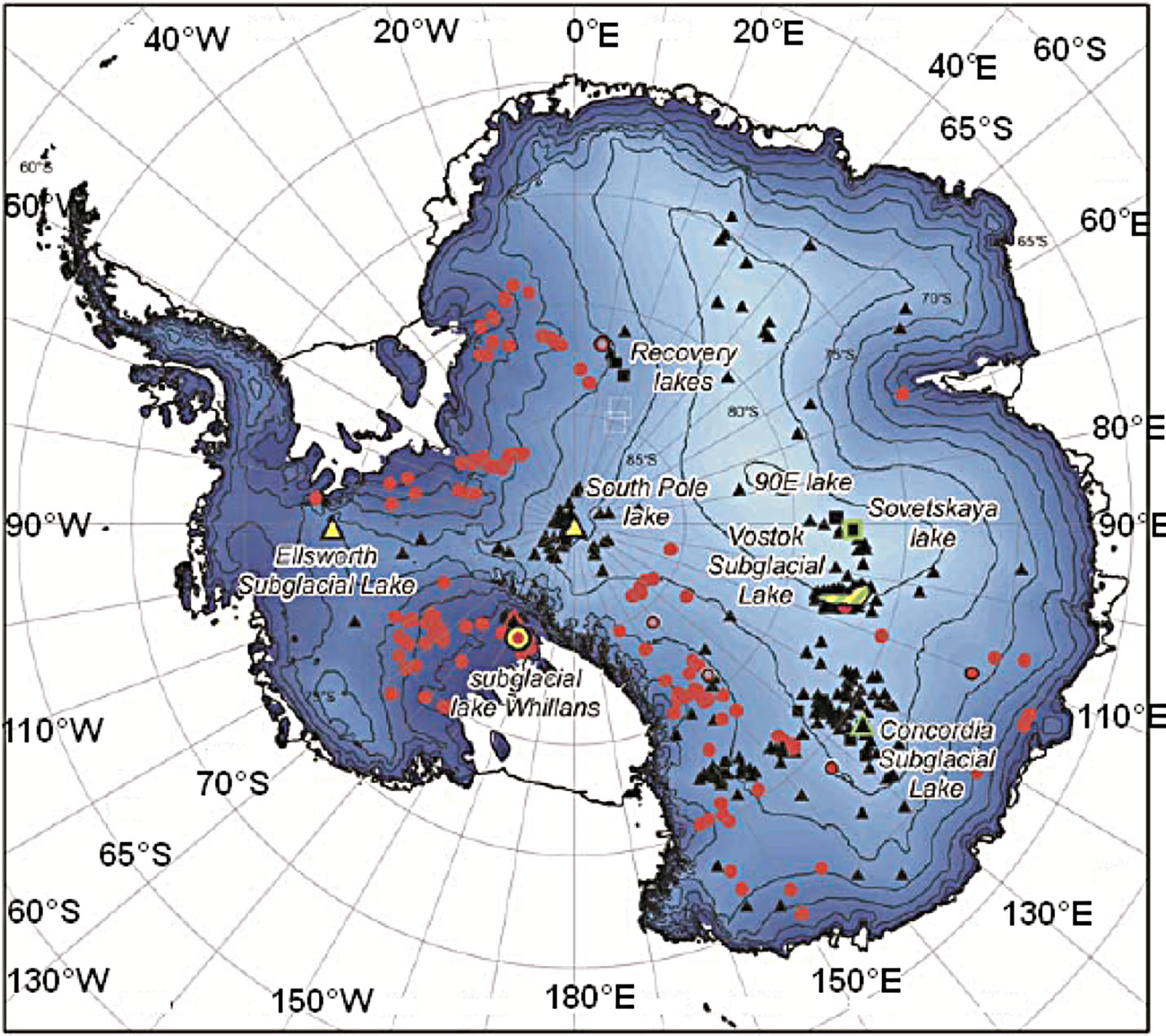
Figure 4. Map of Antarctica showing the locations of all lakes included in the current inventory. Colors/shapes indicate the type of investigations undertaken at each site. Black/triangle: Radio echo sounding; yellow: seismic sounding; green: gravitational field mapping; red/circle: surface height change measurement; square shape identified from ice surface feature. Vostok Lake is shown in outline. After ref. [73].
The largest annual warming trend of 0.56˚C/decade during 1951-2000 has been reported for the western and northern parts of the Antarctic Peninsula. The largest warming of 5˚C over 50 years has been reported at Vernadksy station (former Faraday) (65˚15'S, 64˚16'W) during winter season due to a decrease in winter sea ice over Amundsen-Bellingshausen Sea and increase in ocean-toatmosphere heat fluxes in the winter [79,80]. The West Antarctic warming has been attributed in part to warming in the tropical Pacific Ocean and associated teleconnections [81,82] which are discussed in the next section. The greatest warming during austral summer has occurred on the eastern Peninsula, which is thought to be associated with the enhancement of the circumpolar westerlies over the Southern Ocean (SO), with the Southern Hemisphere Annular Mode (SAM) switching over to its positive phase since the mid-1970s [83]. Stronger winds have facilitated relatively warm, maritime air masses crossing the Peninsula and reaching the low-lying ice shelves on the eastern Peninsula, as well as the adiabatic descent and warming of these winds crossing the Antarctic Peninsula topography [83]. There have been few statistically significant changes in surface air temperature over the last 50 years around the coastal Antarctica. However, a statistically significant cooling in recent decades has been reported for Amundsen-Scott Station (90˚S, 0˚) which is thought to be a result of fewer maritime air masses penetrating into the interior of the continent. Reconstruction of temperatures over the past 200 years, based on eight records distributed over the ice sheet, reveal a warming of 0.2˚C for the past century with no discernible trend [84].
Summertime warming on the eastern side of the Peninsula due to the factors aforementioned has played a major role in the collapse of several ice sheets in this region [85]. In early 1995, a smaller ice shelf area, called the Larsen A, completely disintegrated during a single storm after years of gradually shrinking. On 31st January, 2002, a 3250-square-kilometer section of the Larsen B Ice Shelf rapidly disintegrated into many small fragments in a 35-day period, releasing 500 billion tonnes of ice into the SO (Figure 5). Since 1995, the Larsen Ice Shelf has lost more than 75% of its former area in a series of rapid disintegrations [86]. During March 2008, the Wilkins Ice Shelf in Antarctica retreated by more than 400 square kilometers. Overall in the Antarctic Peninsula, the extent of seven ice shelves declined by a total of about 13,500 square kilometers since 1974. The total ice mass loss for the six glaciers (Hektoria, Green, Evans, Crane, Flask and Lepparde) that feed these ice shelves, exceeded 25 km3/yr and 27 km3/yr for Drygalski Glacier which is located on the northeast tip of the Antarctic Peninsula [87]. During the past 40 years the average summer air temperatures of the northeast Peninsula has been 2.2˚C. It is the warmer air and water temperatures that cause an increased melt on the ice shelf surface, forming ponds of melt water. As the water trickles down through small
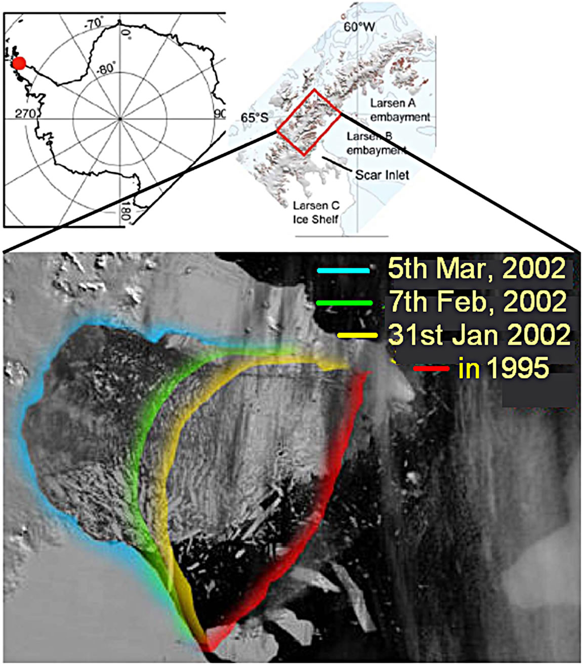
Figure 5. Composite Landsat images with a depiction of maximum ice extents of the Larsen B ice shelf between January and March 2002, relative to the boundary in 1995. Source: NASA.
cracks in the ice shelf, it deepens and erodes, and expands the cracks as it refreezes during the winter. In a separate process, especially in the East Antarctica, warmer ocean water melts the ice shelf from below, thinning it and making it more vulnerable to cracking. Other than these two processes, waning sea ice surrounding the Antarctic Peninsula has also contributed to the recent collapses. Sea ice provides a layer of protection between an ice shelf and the surrounding ocean, muting the power of large waves and storms. As sea ice decreases, more waves buffet the ice shelves. The largest waves can buckle and bend an ice shelf, increasing instability and possibly contributing to its collapse. A decrease in the sea ice also facilitates heat flow from atmosphere to open water thereby, accelerating the thinning of ice sheet from below.
The breakup of other shelves in the Antarctic could have a major effect on the rate of ice flow off the continent. Ice shelves act as braking system for glaciers. Further, the shelves keep warmer marine air at a distance from the glaciers; therefore, they moderate the amount of melting that occurs on the glaciers’ surfaces. Once their ice shelves are removed, the glaciers increase in speed due to melt water percolation and/or a reduction of braking forces, and they may begin to dump more ice into the ocean than they gather as snow in their catchments. Glacier ice speed increases are already observed in peninsular areas where ice shelves disintegrated in prior years.
The collapse of Antarctic ice shelves such as Larsen B on the Antarctic Peninsula does not contribute directly to sea-level change, as they are already floating. However, their vanishing can cause previously dammed glaciers to accelerate and contribute to the sea-level rise. As warming spreads south, the Larsen C ice shelf is beginning to thin and may meet the same fate (Figure 5). Numerically modeled changes of each of the world’s 300,000 glaciers indicate that between 1902 and 2009, melting glaciers contributed 11 cm to sea level rise and are expected to contribute an additional 22 cm until 2100 [88].
Antarctic ice mass balance, which is critical in understanding the global climate and sea-level rise, has long been a controversial topic because of difficulties in estimating it due to lack of reliable data. Hence, space-borne platforms have been used to monitor the state of glaciers. Over the last 50 years, 87% of the 244 glaciers around the coast of the peninsula had retreated and that the average retreat rates have accelerated [89]. The second major area where change has been observed in the Thwaites Glacier and Pine Island (West Antarctica) where the largest discharge of 75 Gt/yr of ice into the SO have been estimated. Different satellite-based techniques were used to address the mass balance. Satellite altimeter observations which records elevation change have indicated a major thinning of the ice sheet in the Pine Island region [90] and the retreat of the grounding line by 5 km inland, between 1992 and 1996, has been inferred from satellite radar interferometry data [91]. Using the altimeter observations an ice mass rate for the whole continent has been in the range of −5 to 85 Gt/yr for the period 1992-2003 [90]. Satellite altimeter measurements are limited by spatial and temporal coverage and by uncertainties in snow density. Using an improvised technology involving interferometric synthetic aperture radar (InSAR), Ref. [92] pointed out that the Antarctic ice loss have increased by 75% from 1996 to 2006, with 196 ± 92 Gt lost in 2006 alone. Further improvement in estimates were possible by using advanced space-based monthly measurements from the Gravity Recovery and Climate Experiment (GRACE) which monitors changes in gravity—an indicator of mass-change at with a spatial resolution of better than a few hundred kilometers, exceeding the scale of most glacial drainage basins. Using these observations from 2002 to January 2009, Chen et al. [93] estimated a significant ice loss of −132 ± 26 Gt/yr for West Antarctic Ice Sheet and −57 ± 52 Gt/yr for East Antarctic Ice Sheet. The largest ice loss of −110.1 Gt/yr was observed in the Amundsen Sea Embayment, followed by the Antarctic Peninsula at −38.1 Gt/yr with most (−28.6 Gt/yr) in its northern part (Graham Land) and the rest (−9.5 Gt/yr) from Alexander Island and nearby regions. The Wilkes Land and Victoria Land had mass loss of −13.4 and −13.1 Gt/yr, respectively. The coastal region in Queen Maud Land showed an ice loss of 6.5 Gt/yr.
6. Low-Latitude Teleconnections with Antarctic Climate
Antarctica is dominantly influenced by remote forcing. The pressure gradient between the higher pressure zone (40˚S - 45˚S) and the low-pressure belt centered on 65˚ is known as the Southern Annular Mode (SAM) or Antarctic Oscillation (AAO). It varies on annual to inter-annual time scales [94]. The SAM reflects north-south meanders in the Southern Hemisphere eddy driven jet, and is strongly related to fluctuations in surface winds and temperatures throughout the high latitude Southern Hemisphere. When the pressures increase at mid-latitudes and decrease at high latitudes, the SAM index, which is the principal mode of variability of the atmospheric circulation of the high latitudes, is in positive phase, and the westerlies are at their strongest. In SAM positive winters, mesocyclones occur frequently through Drake Passage, whereas a latitudinally split pattern is evident there in negative SAM winters [95]. The SAM index fluctuates throughout the year and from year to year. Over the last 50 years it has shifted to its positive phase during the austral summer and autumn, intensifying the westerlies over the SO, greater zonally-averaged sea-ice extent, cooling of most of Antarctica except for the western Antarctic Peninsula. In the latter location, the strong warming and reduced sea-ice extent can be at least partly explained by more frequent north-westerly winds connected to the strengthened SAM. Some modeling studies attribute the development of a positive SAM in the austral summer in recent years to strengthening of the ozone hole, while others suggest that it is caused by greenhouse gas increases. Alternatively, it may be a response to both types of forcing.
The changes in the Antarctic sea-ice concentrations based on the linear regression with the AAO index suggest a wave-number 3 pattern, with a pronounced dipole pattern between the eastern Ross/Amundsen Sea with more sea ice and the Bellingshausen/northern Weddell Sea with less sea ice [96]. These authors demonstrate that with one positive unit of deviation change in the AAO, the sea ice increases (decreases) by about 3% - 7% in the eastern Ross/Amundsen Sea (the Bellingshausen/northern Weddell Sea), which is consistent with the surface cooling (warming) on the magnitude of about 0.5˚C - 2˚C corresponding with the positive phases of the AAO. The response of the Antarctic sea ice to the AAO is a conesquence of a combination of the anomalous mean surface heat flux and ice advection which can be explained as follows. During the high-index polarities of the AAO, an anomalous strong cyclonic circulation in the southeast Pacific leads to an anomalous equatorward (poleward)
mean heat flux at the surface in the Ross/Amundsen Sea (the Bellingshausen/Weddell Sea), which facilitates (limits) sea ice growth. In the Ross/Amundsen sector, an anomalous strong intensification of the surface westerlies associated with the positive phases of the AAO induces an enhanced Ekman drift to the north. The enhanced northward Ekman drift transports cold water equatorward, reducing the oceanic poleward heat transport. The enhanced northward Ekman drift also leads to enhanced equatorward ice advection especially during the cold season because the ice is reduced to the Antarctic continents in summer. The northward dispersion of ice decreases ice thickness and provides more open water for new ice formation in the southern Ross Sea. The newly formed ice is then advected northward by the enhanced Ekman drift, thereby increasing ice cover and thickness further north (the northeast Ross Sea). There is also ice divergence away from both sides of the Antarctic Peninsula (particularly the west side). The contribution of the strong anomalous poleward mean surface heat flux and ice divergence west of the Antarctic Peninsula explain why the maximum warming associated with the positive AAO index occurs there.
El Niño-Southern Oscillation (ENSO) is the dominant global-scale teleconnection, originating in ocean-air interactions in the tropical Pacific [97]. The ENSO teleconnection to high latitudes in the Southern Hemisphere occurs primarily as a standing wave train of anomalies that extends south-eastward through the Amundsen and Bellingshausen seas, crosses the Antarctic Peninsula, and projects into the south-west Atlantic; or Pacific-South America pattern [98]. Instrumental records reveal that ENSO warm events are associated with enhanced precipitation in West Antarctica. West Antarctic precipitation was positively correlated with the Southern Oscillation Index (SOI), until about 1990, after which the two became strongly anti-correlated. The decadal variability of the high latitude ENSO teleconnection to the South Pacific is governed by the phase of the SAM [99]. When both are in the same phase (i.e., La Niña occurring with positive phases of the SAM and vice-versa), the telecomnection is amplified; the connection is much weaker when these two modes are out of phase. During El Niño events (warm Pacific equator), which recur about every four years, high air pressure, warm sea surface temperature and less sea ice often occur west of the Antarctic Peninsula in the Pacific sector, while cold sea surface temperature and more sea ice occur east of the Peninsula in the Atlantic sector. It is also stormier east of the Peninsula than to the west. The opposite conditions apply during intervening La Niña events when equatorial Pacific Ocean cools.
The variation in the Antarctic sea ice with one positive unit of deviation change in the Niño3 index suggest a wave-number 2 pattern, with an increase (decrease) of sea ice in the eastern Ross/Amundsen Sea (the Bellingshausen/Weddell Sea) of similar magnitude (3% - 7%). The mechanisms how the ENSO manifests itself in the Antarctic sea ice can be elucidated as follows [96]. During El Niño events, the intensification (relaxation) of the Hadley Cell in the eastern equatorial Pacific (tropical Atlantic) due to an increased (decreased) pole-to-equator meridional temperature gradient leads to an equatorward (poleward) shift of the subtropical jet. This results in an equatorward (poleward) shift of the storm track in the Ross/Amundsen Seas (the eastern Bellingshausen/Weddell sector). The reduced (enhanced) storm activity in the Ross/Amundsen sector (the eastern Bellingshausen/Weddell sector) leads to a strengthening (weakening) of the poleward segment of the regional Ferrel Cell and a weakening (strengthening) of the equatorward regional Ferrel Cell there, indirectly by changing the meridional eddy heat flux convergence/divergence, and shifting the latent heat release zone. The changes of the regional Ferrel Cell cause anomalous southward (northward) mean meridional heat flux into the sea ice zone in the Ross/Amundsen sector (the eastern Bellingshausen/Weddell sector), which limits (encourages) sea ice growth there. Furthermore, a shift or change of tropical general circulation related to the ENSO variability could perturb the regional mean meridional circulation, thus communicating the changes to high southern latitudes.
The switch of the SAM into more positive conditions and the consequent strengthening of the circumpolar vortex in the recent years is thought to provide arid conditions over large parts of West Antarctica, the Ross Ice Shelf and the Lambert Glacier region, and wetter conditions elsewhere [100]. However, in situ measurement of precipitation on the continent is very difficult, and much of our knowledge of precipitation variability and change has come from ice cores, from which it can be difficult to determine seasonal change. A major study into changes in Antarctic accumulation [101] concluded that there had been no statistically significant change in accumulation across the continent since the International Geophysical Year. However, on longer timescales, and for limited areas, there are indications of change. For example, a new ice core from the south-west corner of the Antarctic Peninsula has shown that there has been a doubling of the accumulation in that region since about 1850 [102].
7. Future Climate Scenario
The coupled atmosphere-ocean climate models are main tools to predict the scenario for the Antarctic region in particular and the Earth in general for the next 100 years. Great efforts are required to implement key physics related to sea ice, cryosphere-ocean-atmosphere interaction and polar stratospheric cloud forcing in the current climate models. The model projections of Antarctic climate over the 21st century reported in the Ref. [103] can be summarized below. The models were run with CO2 double that of the present atmosphere over the next century (up to 2100). The variation expected of the key climate parameters over Antarctica are as follows. Surface temperature would increase by 0.24˚C ± 0.10˚C per decade in the sea ice zone. An overall decrease in sea ice area would be expected (33% ± 9%). An increase in the air temperature by 0.34˚C ± 0.10˚C per decade over the interior of Antarctica and weakening of katabatic winds, particularly during the austral summer season.
Synoptic scale analysis of IPCC model results reveal an increased cyclone activity and stronger zonal winds due to enhanced positive SAM index during the 21st century in Antarctica [104]. With the higher moistureholding capacity of the warmer atmosphere projected for the 21st century, the models predicted an increase of Antarctic precipitation that averages 0.42 ± 0.01 mm/yr [1]. The increased snowfall on the floating ice shelves would weighs them down, making them sink more heavily in the water, while the snowfall on the landmass of Antarctica would increase the elevation toward the interior of the continent. This would result in a steep slope from interior to the coast, thereby enhancing the speed of ice flow up to three times from continent toward the sea, raising the sea-level by 1.25 m in the year 2500, envisaging a warmest scenario [105].
In the scenario of stronger and positive SAM index, enhancement of westerly winds over the SO is expected to isolate Antarctica thereby, preventing penetration of warm maritime air masses in the interior; so lesser warming in the interior of Antarctica is predicted. The extent and thickness of Antarctic ice sheets are expected to implore massive responses, similar to the retreat of Northern Hemisphere ice sheets. Potential impacts of threshold effects on the ice sheet and sea ice extent could result in massive restructuring of the cryosphere-ocean-atmosphere system, triggering rapid climate change events, similar to those experienced during last glacial and current interglacial period.
Paleolimnological studies are also focused on changes in lake salinity from which the atmospheric moisture budget can be inferred and compared with the evidence from Antarctic ice cores. Other studies are required to track the origin and development of the lake biota and, from this, inferences about the nature and direction of environmental change could be inferred. Despite clear signs of marked recent environmental changes over the continent, we have only a limited perspective on how Antarctic climate and environmental conditions have varied in the past. As long-term monitoring programs in high-latitude regions have only been established for the past several decades, paleolimnological methods will continue in developing our understanding of the past environmental changes that will help us anticipate the magnitude, nature, and direction of future change.
8. India’s Contribution to Antarctic Research
India landed on Antarctica on 9th January 1982 and established a base camp on the ice-shelf. In 1983-84, a permanent station Dakshin Gangotri (70˚5'37"S, 12˚E) was established and commissioned on the ice shelf, off the Princess Astrid coast in Central Dronning Maud Land. India built a second permanent station Maitri (70˚45'57"S, 11˚44'09"E; 117 m above mean sea level) on Schirmacher Oasis situated on Queen Maud Land, East Antarctica, during 1988-89, as the first research station got buried under ice. The Ministry of Earth Sciences (former Department of Ocean Development), Government of India, established on the 25th May 1998, the National Centre for Antarctic and Ocean Research (NCAOR) to handle polar research and logistic activities (http://www.ncaor.gov.in). A third state-of-art Bharti station (69˚24'28'S, 76˚11'14"E; 43 m above mean sea level) was raised during 2011-12 at unnamed promontory between Stornes and Broknes Peninsula in the Larsemann Hills. It is about 3000 km from Schirmacher Oasis where station Maitri stands.
The Indian Antarctic program involves multi-institutions and multidisciplinary researchers with broad themes focused on the following topical areas: Meteorology and Atmospheric Sciences, Earth Sciences and Glaciology, Environment and Biological Sciences, Engineering and Communication, Human Physiology and Medicine, and Southern Ocean Oceanography. The Indian Meteorological Department has established an uninterrupted data set spanning more than three decades. The air temperature during 1991-2010 indicated a cooling trend of −0.4˚C/ decade. During the same period wind speed showed an increasing trend of 0.27 kt/decade, with a decreasing trend of −0.43 kt/decade during 2001-2010; the latter is as a result of less cyclonic disturbances affecting Maitri [106]. It has been shown that negative SAM index leads warmer surface temperature in the central Dronning Maud Land [106]. Measurements of ozone concentration using Brewer Ozone Spectrophotometer showed that it varied by 4% in during 2005-06 and 2006-07 summer period [107].
Geomagnetospheric measurements consisting of atmospheric electricity parameters and their response to the global thunderstorm activity and space weather events have been carried at Maitri station. Though Maitri is at the equatorial peripheral of the Auroral electrojet, during the geomagnetic storm the station comes under the influence of the auroral electrojet which enables the field line currents to influence the upper space environment [108]. Ref. [108] suggests the existence of correlation between the atmospheric electrical parameters and geomagnetic activity. Indian geologists have mapped about 20,000 sq km of the area in central Dronning Maud land on a 1:50,000 scale. Three geological maps of Schirmacher Oasis, Wohlthat and Orvin Mountains and a geomorphological map of Schirmacher Oasis are published (www.portal.gsi.gov.in). Monitoring of glacier snout and the continental ice margin adjoining India Bay in Princess Astrid Coast, on a regular basis has revealed significant retreat of the ice margin in the last two decades [109].
Shallow ice coring (<100 m) has been conducted to reconstruct the Antarctic paleoclimatic and environmental conditions. The snow samples and ice core packed in polythene containers and shipped in deep-freezers, which are analysed at a state-of-art ice core repository-cumlaboratory at NCAOR. Ice cores drilled from the continental ice, south of Maitri, has been analyzed to evaluate the temporal changes in environmental characteristics during past few centuries. Based on δ18O measurements on a 30 m ice core raised from east Antarctica (70˚47'S, 11˚44'E), the mean annual surface air temperatures data observed during the last 150 years indicates that the beginning of the 19th century was cooler by about 2˚C than the recent past and the middle of 18th century [110]. Using 210Pb and δ180, the mean annual accumulation rates were found to be 20 and 21 cm of ice equivalent per year, respectively. An Analysis of a 62.2 m core from Central Dronning Maud Land (70˚51.3'S, 11˚32.2'E) representing last five centuries revealed non-sea salt sulfate aerosol deposition during large volcanic eruption events like Mt Pinatubo in 1991, Agung in 1963, Krakatau/Tarawera in 1883/1886, Tambora in 1815 and Huaynaputina in 1600 [111]. The nitrate profile reveals a systematic negative shift since the mid-18th century, suggesting a possible change in the zonal wind transport and an apparent solar modulation of the same [112].
Around 125 new species of psychrophilic microbes have been discovered of which India has contributed around 20 new species [113-117]. Refs. [118,119] identified two new species of psychrophilic microbes christened as Arthobacter Gangotriensis and Planococcus Maitriensis after Indian station Dakshin Gangotri and Maitri, respectively. Genomic studies indicated that the genes involved in protein synthesis and amino acid metabolism were found to be essential for the survival of the micro-organisms at temperatures below 10˚C. These microbes are cultured to generate as enzymes or bio-molecules with application in biotech industry, medicine and agriculture. Indian Antarctic stations have provided a platform for collaborative studies with some Antarctic Treaty nations such as Germany, Italy, France, Poland and the USA. These stations have also facilitated scientists from Malaysia, Columbia, Peru and Mauritius to work in Antarctica.
9. Conclusions
Antarctica is a barometer of the Earth’s climate system which records signatures of global climate change induced by local (anthropogenic) and remote forcing. Antarctic modern climate evolves through an interaction of cryosphere-ocean-atmosphere system in response to past and present climate forcing. Superimposed on the longterm trend of post-glacial warming are millennial and finer scale oscillations, for example, those associated with the 11-year sunspot cycle.
In the last 50 years, the near-surface air temperature has risen over the west of the Antarctic Peninsula, concomitant with an increase in sea surface temperature, retreat of glaciers and the collapse of ice shelves around the Antarctic Peninsula. The SAM index has switched over to positive mode in the last five decades leading to the intensification and southward shift of the westerlies over the SO, and warming of the west Antarctica, mostly the Antarctic Peninsula. On the other hand, cooling of the stratosphere over Antarctica has enhanced the development of polar stratospheric clouds thereby, intensifying the ozone depletion. As for the ice loss, East Antarctica is stable compared to the Antarctic Peninsula and West Antarctica. The inhomogeneity of Antarctic climate in space and time implies that recent Antarctic climate changes are due on the one hand to a combination of strong multidecadal variability and anthropogenic effects and, as demonstrated by the paleoclimate record, on the other hand to multidecadal to millennial scale and longer natural variability forced through changes in orbital insolation, greenhouse gases, solar variability, ice dynamoics, and aerosols.
The scenario of Antarctic climate changes in the 21st century projects warming of the sea ice zone, reduction in sea ice extent, warming of the Antarctic Plateau, and increased precipitation in snow form. Climate models needs to incorporate better atmospheric physics and glacier dynamics to forecast the change at the regional level. The retreat of the Antarctic ice sheet since the Last Glacial Maximum could be significantly accelerated by global warming. Ice sheet models are inadequately represented with the mechanisms related to the effect of warming on ice melt and subsequent sea level rise. Threshold effects may have a significant impact on the ice sheet and sea ice extent. During the last glacial and current interglacial, such effects resulted in massive reorganizations of the cryosphere-ocean-atmosphere system, leading to rapid climate change events. Comprehensive satellite data reinforced by ground truth, and modeling of the oceanice-atmosphere system are needed to forecast and quantify climate change with confidence on regional and global scales.
Some recommendations for future studies are as follows: 1) Observational program for Antarctica should be taken on a larger scale. A high accurate meteorological, glaciological and environmental chemistry data are needed for determining the trends and their statistical significance. Automatic Weather Stations should be installed in remote locations, especially in the Antarctic Plateau. 2) With the available and now assemblage of time series from several sources, it is necessary to maintain an appropriate data archive, such that all of the existing data (plus future data) can be easily accessed and utilized by individual researchers and institutions. Provisions should also be made so that data available in the future from newer instrumentation and/or observing platforms can be added to the archive with relative ease. 3) The variability on different scales, ranging from monthly to seasonal to annual to interannual to decadal, and spatial scales ranging from individual locations to regional areas to zonal belts to planetary dimensions, needs to be fully documented. In this regard, further work is needed on understanding and modeling the effects of variations due to solar irradiance changes, volcanic eruptions, Indian Ocean Dipole, ENSO, quasi-biennial zonal wind oscillation in order to improve upon the estimates of natural variability, such that trends detection and in particular their attribution to anthropogenic causes.
Circulation model experiments on global scale are needed to explore further the dynamical effects influencing the temperature structure of the stratosphere (e.g., responses to greenhouse gas increases which lead to a change in the tropospheric equator-to-pole heating gradient and planetary wave propagation) and to what extent they can alter the stratospheric circulation. Such studies should continue to make comparisons with appropriate diagnostics of up-to-date observations so that the influences on circulation can be accurately quantified. 4) The biodiversity has significant gradients which can be defined on the basis of latitude, altitude and depth. The distribution patterns and biodiversity in the terrestrial and marine ecosystems of Antarctica are governed by temperature, water, ice cover, oxygen and light, respectively. The alien invaders among animals comprise bryozoans, barnacles, polychaete worms, hydroids, crabs and mollusks, whereas grasses such as Avena, Plantago and Poa have been reported as alien plants from Marion Island. An estimated 18 vascular plants have taken root in Antarctica as a result of human activities. There is need for an internationally coordinated programme to map the alien species promoted by visitors, the impact of ultraviolet-B induced changes on flora and fauna, and predict the consequences arising out of global changes such as increasing atmospheric carbon dioxide and surface warming on earth’s biosphere.
10. Acknowledgements
I thank Director, Dr. S. Rajan, for his support and encouragement. This is NCAOR contribution 11/2013.
REFERENCES
- P. Uotila, A. H. Lynch, J. J. Cassano and R. I. Cullather, “Changes in Antarctic Net Precipitation in the 21st Century Based on Intergovernmental Panel on Climate Change (IPCC) Model Scenarios,” Journal of Geophysical Research, Vol. 112, No. D10, 2007, Article ID: D10107. doi:10.1029/2006JD007482
- P. R. Holland and R. Kwok, “Wind-Driven Trends in Antarctic Sea-Ice Drift,” Nature Geoscience, Vol. 5, No. 12, 2012, pp. 872-875.
- A. Wegner, “The Origin of Continents and Oceans,” Methuen and Co. Ltd., London, 1924.
- R. M. DeConto and D. Pollard, “Rapid Cenozoic Glaciations of Antarctica Induced by Declining Atmospheric CO2,” Nature, Vol. 421, No. 6920, 2003, pp. 245-249.
- M. Pagani, J. Zachos, K. H. Freeman, B. Tipple and S. M. Boharty, “Marked Decline in Atmospheric Carbon Dioxide Concentrations during the Paleogene,” Science, Vol. 309, No. 5734, 2005, pp. 600-603.
- J. C. Zachos, J. R. Breza and S. W. Wise, “Early Oligocene Ice Sheet Expansion on Antarctica, Sedimentological and Isotopic Evidence from the Kergulen Plateau,” Geology, Vol. 20, No. 6, 1992, pp. 569-573.
- B. P. Flower and J. P. Kennett, “The Middle Miocene Climatic Transition: East Antarctic Ice Sheet Development, Deep Ocean Circulation and Global Carbon Cycling,” Palaeogeography, Palaeoclimatology, Palaeoecology, Vol. 108, No. 3-4, 1994, pp. 537-555.
- J. C. Farman, B. G. Gardiner and J. D. Shanklin, “Large Losses of Total Ozone in Antarctica Reveal Seasonal ClOx/NOx Interaction,” Nature, Vol. 315, 1985, pp. 207- 210. doi:10.1038/315207a0
- P. Hamill and O. B. Toon, “Polar Stratospheric Clouds and the Ozone Depletion,” Physics Today, Vol. 44, No. 12, 1991, pp. 34-42. doi:10.1063/1.881277
- World Meteorological Organization Global Ozone Research and Monitoring Project, “Scientific Assessment of Ozone Depletion: 2006,” Report 50, World Meteorological Organization, Geneva, 2007.
- D. W. J. Thompson and S. Solomon, “Interpretation of recent Southern Hemisphere Climate Change,” Science, Vol. 296, No. 5569, 2002, pp. 895-899. doi:10.1126/science.1069270
- G. J. M. Velders, S. O. Andersen, J. S. Daniel, D. W. Fahey and M. McFarland, “The Importance of the Montreal Protocol in Protecting Climate,” Proceedings of the National Academy of Sciences of the United States of America, Vol. 104, No. 12, 2007, pp. 4814-4819.
- M. J. Newchurch, E.-S. Yang, D. M. Cunnold, G. C. Reinsel, J. M. Zawodny and J. M. Russell III, “Evidence for Slowdown in Stratospheric Ozone Loss: First Stage of Ozone Recovery,” Journal of Geophysical Research, Vol. 108, No. D16, 2003, Article ID: 4507. doi:10.1029/2003JD003471
- United Nations Framework Convention on Climate Change, “Kyoto Protocol to the United Nations Framework Convention on Climate Change,” 1997.
- S. Hong, Y. Kim, C. F. Boutron, C. P. Ferrari, J. R. Petit, C. Barbante, K. Rosman and Y. Lipenkov, “Climate Related Variations in Lead Concentration and Sources in Vostok Antarctic Ice from 65,000 to 240,000 Years BP,” Geophysical Research Letters, Vol. 30, No. 22, 2003, Article ID: 2138. doi:10.1029/2003GL018411
- C. F. Boutron and C. C. Patterson, “The Occurrence of Lead in Antarctic Recent Snow, Firn Deposited over the Last Two Centuries and Prehistoric Ice,” Geochimica et Cosmochimica Acta, Vol. 47, No. 8, 1983, pp. 1355- 1368.
- E. W. Wolff and E. D. Suttie, “Antarctic Snow Record of Southern Hemisphere Lead Pollution,” Geophysical Research Letters, Vol. 21, No. 9, 1994, pp. 781-784. doi:10.1029/94GL00656
- E. W. Wolff, E. D. Suttie and D. A. Peel, “Antarctic Snow Record of Cadmium, Copper and Zinc Content during the Twentieth Century,” Atmospheric Environment, Vol. 33, No. 10, 1999, pp. 1535-1541.
- F. A. M. Planchon, C. F. Boutron, C. Barbante, G. Cozzi, V. Gaspari, E. W. Wolff, C. P. Ferrari and P. Cescon, “Changes in Heavy Metals in Antarctic Snow from Coats Land since the Mid-19th to the Late-20th Century,” Earth and Planetary Science Letters, Vol. 200, No. 1-2, 2002, pp. 207-222.
- P. Vallelonga, K. van de Velde, J. P. Candelone, I. Morgan, C. F. Boutron and K. J. R. Rosman, “The Lead Pollution History of Law Dome, Antarctica, from Isotopic Measurements on Ice Cores: 1500 AD to 1989 AD,” Earth and Planetary Science Letters, Vol. 204, No. 1-2, 2002, pp. 291-306.
- K. van de Velde, P. Vallelonga, J. P. Candelone, K. J. R. Rosman, V. Gaspari, G. Cozzi, C. Barbante, R. Udisti, P. Cescon and C. Boutron, “Pb Isotope Record over One Century in Snow from Victoria Land, Antarctica,” Earth and Planetary Science Letters, Vol. 232, No. 1-2, 2005, pp. 95-108. doi:10.1016/j.epsl.2005.01.007
- R. Fuoco, M. P. Colombini, A. Ceccarini and C. Abete, “Polychlorobiphenyls in Antarctica,” Microchemical Journal, Vol. 54, No. 4, 1996, pp. 384-390. doi:10.1006/mchj.1996.0115
- S. Corsolini, T. Romeo, N. Ademollo, S. Greco and S. Focardi, “POPs in Key Species of Marine Antarctic Ecosystem,” Microchemical Journal, Vol. 73, No. 1-2, 2002, pp. 187-193.
- K. Weber and H. Goerke, “Persistent Organic Pollutants (POPs) in Antarctic Fish: Levels, Patterns, and Changes,” Chemosphere, Vol. 53, No. 6, 2003, pp. 667-678.
- R. C. Montone, S. Taniguchi and R. R. Weber, “PCBs in the Atmosphere of King George Island, Antarctica,” The Science of the Total Environment, Vol. 308, No. 1-3, 2003, pp. 167-173.
- J. Dibb, P. A. Mayewski, C. F. Buck and S. M. Drummey, “Beta Radiation from Snow,” Nature, Vol. 345, No. 6270, 1990, p. 25.
- A. M. Rankin, V. Auld and E. W. Wolff, “Frost Flowers as a Source of Fractionated Sea Salt Aerosol in the Polar Regions,” Geophysical Research Letters, Vol. 27, No. 21, 2000, pp. 3469-3472. doi:10.1029/2000GL011771
- A. M. Rankin, E. W. Wolff and S. Martin, “Frost Flowers: Implications for Tropospheric Chemistry and Ice Core Interpretation,” Journal of Geophysical Research, Vol. 107, No. D23, 2002, p. 4683. doi:10.1029/2002JD002492
- P. A. Mayewski, M. P. Meredith, C. P. Summerhayes, J. Turner, A. Worby, P. J. Barrett, G. Casassa, N. A. N. Bertler, T. Bracegirdle, A. C. N. Garabato, D. Bromwich, H. Campbell, G. S. Hamilton, W. B. Lyons, K. A. Maasch, S. Aoki, C. Xiao and T. van Ommen, “State of the Antarctic and Southern Ocean Climate System,” Reviews of Geophysics, Vol. 47, No. 1, 2009, Article ID: RG1003. doi:10.1029/2007RG000231
- M. Thamban, C. M. Laluraj, S. S. Naik and A. Chaturvedi, “Reconstruction of Antarctic Climate Change Using Ice Core Proxy Records from the Coastal Dronning Maud Land, East Antarctica,” Journal of the Geological Society of India, Vol. 78, No. 1, 2011, pp. 19-29.
- S. Benassai, S. Becagli, R. Gragnani, O. Magand, M. Proposito, I. Fattori, R. Traversi and R. Udisti, “SeaSpray Deposition in Antarctic Coastal and Plateau Areas from ITASE Traverses,” Annals of Glaciology, Vol. 41, No. 1, 2005, pp. 32-40. doi:10.3189/172756405781813285
- R. Naveen, H. J. Lynch, S. Forrest, T. Mueller and M. Polito, “First Direct, Site-Wide Penguin Survey at Deception Island, Antarctica, Suggests Significant Declines in Breeding Chinstrap Penguins,” Polar Biology, Vol. 35, No. 12, 2012, pp. 1879-1888.
- P. T. Fretwell, M. A. LaRue, P. Morin, G. L. Kooyman, B. Wienecke, N. Ratcliffe, A. J. Fox, A. H. Fleming, C. Porter and P. N. Trathan, “An Emperor Penguin Population Estimate: The First Global, Synoptic Survey of a Species from Space,” PLoS One, Vol. 7, No. 4, 2012, Article ID: e33751. doi:10.1371/journal.pone.0033751
- W. Z. Trivelpiece, J. T. Hinke, A. K. Miller, C. S. Reiss, S. G. Trivelpiece and G. M. Watters, “Variability in Krill Biomass Links Harvesting and Climate Warming to Penguin Population Changes in Antarctica,” Proceedings of the National Academy of Sciences of the United States of America, Vol. 108, No. 18, 2011, pp. 7625-7628. doi:10.1073/pnas.1016560108
- W. Z. Trivelpiece, S. G. Trivelpiece, G. R. Geupel, J. Kjelmyr and N. J. Volkman, “Antarctic Ecosystems-Ecological Change and Conservation,” Springer, Berlin, 1990.
- A. Atkinson, V. Siegel, E. Pakhomov and P. Rothery, “Long-Term Decline in Krill Stock and Increase in Salps within the Southern Ocean,” Nature, Vol. 432, No. 7013, 2004, pp. 100-103.
- IPCC, “Contribution of Work Groups I, II and III to the 4th Assessment Report of the Intergovernmental Panel on Climate Change,” Climate Change Synthesis Report, Geneva, 2007.
- A. Atkinson, V. Siegel, E. A. Pakhomov, P. Rothery, V. Loeb, R. M. Ross, L. B. Quetin, K. Schmidt, P. Fretwell, E. J. Murphy, G. A. Tarling and A. H. Fleming, “Oceanic Circumpolar Habitats of Antarctic Krill,” Marine Ecology Progress Series, Vol. 362, 2008, pp. 1-23. doi:10.3354/meps07498
- V. Loeb, V. Siegel, O. Holm-Hansen, R. Hewitt, W. Fraserk, W. Trivelpiecek and S. Trivelpiecek, “Effects of Sea-Ice Extent and Krill or Salp Dominance on the Antarctic Food Web,” Nature, Vol. 387, No. 6636, 1997, pp. 897-900.
- D. G. Vaughan, G. J. Marshall, W. M. Connolley, C. Parkinson, R. Mulvaney, D. A. Hodgson, J. C. King, C. J. Pusdsey and J. Turner, “Recent Rapid Regional Climate Warming on the Antarctic Peninsula,” Climatic Change, Vol. 60, No. 3, 2003, pp. 243-274. doi:10.1023/A:1026021217991
- M. P. Meredith and J. C. King, “Rapid Climate Change in the Ocean West of the Antarctic Peninsula during the Second Half of the 20th Century,” Geophysical Research Letters, Vol. 32, No. 19, 2005, Article ID: L19604. doi:10.1029/2005GL024042
- F. A. O’Gorman, “Fur Seals Breeding in the Falkland Islands Dependencies,” Nature, Vol. 192, 1961, pp. 914- 916. doi:10.1038/192914a0
- I. L. Boyd, “Pup Production and Distribution of Breeding Antarctic Fur Seals (Arctocephalus gazelle) at South Georgia,” Antarctic Science, Vol. 5, No. 1, 1993, pp. 17- 24. doi:10.1017/S0954102093000045
- J. McClintock, H. W. Ducklow and W. Fraser, “Ecological Responses to Climate Change on the Antarctic Peninsula,” American Scientist, Vol. 96, No. 4, 2008, pp. 302-310. doi:10.1511/2008.73.3844
- J. Forcada, P. N. Trathan, K. Reid, J. Murphy and J. P. Croxall, “Contrasting Population Changes in Sympatric Penguin Species in Association with Climate Warming,” Global Change Biology, Vol. 12, No. 3, 2006, pp. 411- 423. doi:10.1111/j.1365-2486.2006.01108.x
- O. Schofield, H. W. Ducklow, D. G. Martinson, M. P. Meredith, M. A. Moline and W. R. Fraser, “How Do Polar Marine Ecosystems Respond to Rapid Climate Change?” Science, Vol. 328, No. 5985, 2010, pp. 1520- 1523. doi:10.1126/science.1185779
- L. Beyer, M. Bölter and R. D. Seppelt, “Nutrient and Thermal Regime, Microbial Biomass and Vegetation of Antarctic Soils in the Windmill Islands Region of East Antarctica Wilkes Land,” Arctic Antarctic and Alpine Research, Vol. 32, No. 1, 2000, pp. 30-39. doi:10.2307/1552407
- M. Alberdhi, A. León, L. A. Bravo, A. Gutiérrez, M. Gidekelc and L. C. Corcuerab, “Ecophysiology of Antarctic Vascular Plants,” Physiologia Plantarum, Vol. 115, No. 4, 2002, pp. 479-486. doi:10.1034/j.1399-3054.2002.1150401.x
- H. Bednarek-Ochyra, J. Vana, R. Ochyra and R. I. L. Smith, “The Liverwort Flora of Antarctica,” Polish Academy of Sciences, Institute of Botany, Cracow, 2000.
- R. Ochyra, R. I. L. Smith and H. Bednarek-Ochyra, “Illustrated Moss Flora of Antarctica,” Cambridge University Press, Cambridge, 2008.
- D. O. Øvstedal and R. I. L. Smith, “Lichens of Antarctica and South Georgia: A Guide to Their Identification and Ecology,” Cambridge University Press, Cambridge, 2001.
- M. Olech and S. M. Singh, “Lichens and Lichenocolous fungi of Schirmacher Oasis,” National Centre for Antarctic and Ocean Research, Vasco da Gama, 2010.
- A. Taton, S. Grubisic, E. Brambilla, R. de Wit and A. Wilmotte, “Cyanobacterial Diversity in Natural and Artificial Microbial Mats of Lake Fryxell (McMurdo Dry Valleys, Antarctica): A Morphological and Molecular Approach,” Applied and Environmental Microbiology, Vol. 69, No. 9, 2003, pp. 5157-5169. doi:10.1128/AEM.69.9.5157-5169.2003
- Z. Namsaraev, M. J. Mano, R. Fernandez and A. Wilmotte, “Biogeography of Terrestrial Cyanobacteria from Antarctic Ice-Free Areas,” Annals of Glaciology, Vol. 51, No. 56, 2010, pp. 171-177. doi:10.3189/172756411795931930
- K. D. Pandey, S. P. Shukla, P. N. Shukla, D. D. Giri, J. S. Singh, P. Singh and A. K. Kashyap, “Cyanobacteria in Antarctica: Ecology, Physiology and Cold Adaptation,” Cellular and Molecular Biology, Vol. 50, No. 5, 2004, pp. 575-584.
- M. L. Skotnicki, J. A. Ninham and P. M. Selkirk, “High Levels of RAPD Diversity in the Moss Bryum Argenteum in Australia, New Zealand, and Antarctica,” The Bryologist, Vol. 10, No. 3, 1998, pp. 412-421.
- B. Battaglia, J. Valencia and D. W. H. Walton, “Antarctic Communities: Species, Structure, and Survival,” Cambridge University Press, Cambridge, 1997.
- A. Camacho, “Planktonic Microbial Assemblages and the Potential Effects of Metazooplankton Predation on the Food Web of Lakes from the Maritime Antarctica and Sub-Antarctic Islands,” Review in Environmental Science and Biotechnology, Vol. 5, No. 2-3, 2005, pp. 167-185. doi:10.1007/s11157-006-0003-2
- J. C. Ellis-Evans, “Microbial Diversity and Function in Antarctic Freshwater Ecosystems,” Biodiversity and Conservation, Vol. 5, No. 11, 1996, pp. 1395-1431. doi:10.1007/BF00051985
- W. F. Vincent, “Cyanobacterial Dominance in the Polar Regions,” In: B. A. Whitton and M. Potts, Eds., The Ecology of Cyanobacteria: Their Diversity in Time and Space, Academic Press, Dordrecht, 2000, pp. 321-240.
- J. Laybourn-Parry, “The Microbial Loop in Antarctic Lakes,” In: W. B. Lyons, C. Howard-Williams and I. Hawes, Eds., Ecosystem Processes in Antarctic Ice-Free Landscapes, Balkema, Rotterdam, 1997, pp. 231-240.
- K. P. Krishnan, R. K. Sinha, K. Krishna, S. Nair and S. M. Singh, “Microbially Mediated Redox Transformations of Mangnese II. along with Some Other Trace Elements: A Study from Antarctic Lakes,” Polar Biology, Vol. 32, No. 12, 2009, pp. 1765-1778. doi:10.1007/s00300-009-0676-4
- A. B. Paul, “The Ecology of Chasmolithic Algae at Coastal Locations of Antarctica,” Phycologia, Vol. 20, No. 3, 1981, pp. 259-272. doi:10.2216/i0031-8884-20-3-259.1
- Scientific Committee on Antarctic Research, “The Protocol on Environmental Protection to the Antarctic Treaty, with Annexes, Done at Madrid 4 October 1991, and an Additional Annex Done at Bonn, October 1991,” SCAR Bulletin 110, Cambridge, 1993.
- S. L. Chown, A. H. L. Huiskes, N. J. M. Gremmen, J. E. Lee, A. Terauds, K. Crosbie, Y. Frenot, K. A. Hughes, S. Imura, K. Kiefer, M. Lebouvier, B. Raymond, M. Tsujimoto, C. Ware, B. Van de Vijver and D. M. Bergstrom, “Continent-Wide Risk Assessment for the Establishment of Nonindigenous Species in Antarctica,” Proceedings of the National Academy Sciences of the United States of America, Vol. 109, No. 13, 2012, pp. 4938-4943. doi:10.1073/pnas.1119787109
- A. P. Kapitsa, J. K. Ridley, G. Q. Robin, M. J. Siegert and I. A. Zotikov, “A Large Deep Freshwater Lake Beneath the Ice of Central East Antarctica,” Nature, Vol. 381, 1996, pp. 684-686. doi:10.1038/381684a0
- J. C. Priscu, E. E. Adams, W. B. Lyons, M. A. Voytek, D. W. Mogk, R. L. Brown, C. P. McKay, C. D. Takacs, K. A. Welch, C. F. Wolf, J. D. Kirshtein and R. Avci, “Geomicrobiology of Subglacial Ice above Lake Vostok, Antarctica,” Science, Vol. 286, No. 5447, 1999, pp. 2141-2144. doi:10.1126/science.286.5447.2141
- J. A. Dowdeswell and M. J. Siegert, “The Physiography of Modern Antarctic Subglacial Lakes,” Global and Planetary Change, Vol. 35, No. 3-4, 2002, pp. 221-236. doi:10.1016/S0921-8181(02)00128-5
- H. J. Zwally, B. Schutz, W. Abdalati, J. Abshire, C. Bentley, A. Brenner, J. Bufton, J. Dezio, D. Hancock, D. Harding, T. Herring, B. Minster, K. Quinn, S. Palm, J. Spinhirne and R. Thomas, “ICESat’s Laser Measurements of Polar Ice, Atmosphere, Ocean, and Land,” Journal of Geodynamics, Vol. 34, No. 3-4, 2002, pp. 405-445. doi:10.1016/S0264-3707(02)00042-X
- T. Schenk, B. Csatho, C. J. van der Veen, H. Brecher, Y. Ahn and T. Yoon, “Registering Imagery to ICESat Data for Measuring Elevation Changes on Byrd Glacier, Antarctica,” Geophysical Research Letters, Vol. 32, No. 23, 2005, Article ID: L23S05. doi:10.1029/2005GL024328
- T. Schenk and B. Csatho, “A New Methodology for Detecting Ice Sheet Surface Elevation Changes from Laser Altimetry Data,” Geoscience and Remote Sensing, Vol. 50, No. 9, 2012, pp. 3302-3316. doi:10.1109/TGRS.2011.2182357
- M. J. Siegert, S. Carter, I. Tabacco, S. Popov and D. D. Blankenship, “A Revised Inventory of Antarctic Subglacial Lakes,” Antarctic Science, Vol. 17, No. 3, 2005, pp. 453-460. doi:10.1017/S0954102005002889
- A. Wright and M. Siegert, “A Fourth Inventory of Antarctic Subglacial Lakes,” Antarctic Science, Vol. 24, No. 6, 2012, pp. 659-664. doi:10.1017/S095410201200048X
- T. Pavel, “Russian Researchers Reach Subglacial Lake Vostok in Antarctica,” Advances in Polar Science, Vol. 23, No. 3, 2012, pp. 176-180.
- P. T. Doran, J. C. Priscu, W. B. Lyons, R. D. Powell, D. T. Andersen and R. J. Poreda, “Paleolimnology of Extreme Cold Terrestrial and Extraterrestrial Environments,” In: R. Pienitz, M. S. V. Douglas and J. P. Smol, Eds., Developments in Palaeoenvironmental Research, Springer, Dordrecht, 2004, pp. 475-507.
- J. Turner, T. A. Lachlan-Cope, S. R. Colwell, G. J. Marshall and W. M. Connolley, “Significant Warming of the Antarctic Winter Troposphere,” Science, Vol. 311, No. 5769, 2006, pp. 1914-1917. doi:10.1126/science.1121652
- V. Ramaswamy, M.-L, Chanin, J. Angell, J. Barnett, D. Gaffen, M. Gelman, P. Keckhut, Y. Koshelkov, K. Labitzke, J.-J Lin, A. O’Neill, J. Nash, W. Randel, R. Rood, K. Shine, M. Shiotani and R. Swinbank, “Stratospheric Temperature Trends: Observations and Model Simulations,” Reviews of Geophysics, Vol. 39, No. 1, 2001, pp. 71-122. doi:10.1029/1999RG000065
- K. P. Shine, M. S. Bourqui, P. M. de F. Forster, S. H. E. Hare, U. Langematz, P. Braesicke, V. Grewe, M. Ponater, C. Schnadt, C. A. Smith, J. D. Haigh, J. Austin, N. Butchart, D. T. Shindell, W. J. Randel, T. Nagashima, R. W. Portmann, S. Solomon, D. J. Seidel, J. Lanzante, S. Klein, V. Ramaswamy and M. D. Schwarzkopf, “A Comparison of Model-Simulated Trends in Stratospheric Temperatures,” Quarterly Journal of Royal Meteorological Society, Vol. 129, No. 590, 2003, pp. 1565-1588. doi:10.1256/qj.02.186
- J. Turner, S. A. Harangozo, J. C. King, W. M. Connolley, T. A. Lachlan-Cope and G. J. Marshall, “An Exceptional Winter Sea-Ice Retreat/Advance in the Bellingshausen Sea, Antarctica,” Atmosphere-Ocean, Vol. 41, No. 2, 2003, pp. 171-185. doi:10.3137/ao.410205
- J. Turner and J. Overland, “Contrasting Climate Change in the Two Polar Regions,” Polar Research, Vol. 28, No. 2, 2009, pp. 146-164. doi:10.1111/j.1751-8369.2009.00128.x
- Q. Ding, E. J. Steig, D. S. Battisti and M. Kuttel, “Winter Warming in West Antarctica Caused by Central Tropical Pacific Warming,” Nature Geoscience, Vol. 4, No. 6, 2011, pp. 398-403.
- D. P. Schneider, Y. Okumura and C. Deser, “Observed Antarctic Interannual Climate Variability and Tropical Linkages,” Journal of Climate, Vol. 25, No. 12, 2012, pp. 4048-4066. doi:10.1175/JCLI-D-11-00273.1
- G. J. Marshall, A. Orr, N. P. M. Van Lipzig and J. C. King, “The Impact of Changing Southern Hemisphere Annular Mode on Antarctic Peninsula Summer Temperatures,” Journal of Climate, Vol. 19, No. 20, 2006, pp. 5388-5404. doi:10.1175/JCLI3844.1
- D. P. Schneider, E. J. Steig, T. D. van Ommen, C. M. Bitz, D. Dixon, P. A. Mayewski and J. M. Jones, “Antarctic Temperatures over the Past Two Centuries, from Ice Cores,” Geophysical Research Letters, Vol. 33, No. 16, 2006, Article ID: L16707. doi:10.1029/2006GL027057
- T. A. Scambos, C. Hulbe, M. A. Fahnestock and J. Bolander, “The Link between Climate Warming and Breakup of Ice Shelves in the Antarctic Peninsula,” Journal of Glaciology, Vol. 46, No. 154, 2000, pp. 516- 530. doi:10.3189/172756500781833043
- T. A. Scambos, J. Bohlander, C. Shuman and P. Skvarca, “Glacier Acceleration and Thinning after Ice Shelf Collapse in the Larsen B Embayment, Antarctica,” Geophysical Research Letters, Vol. 31, No. 18, 2004, Article ID: L18402. doi:10.1029/2004GL020670
- E. J. Rignot, G. Casassa, P. Gogineni, W. Krabill, A. Rivera and R. Thomas, “Accelerated Ice Discharge from the Antarctic Peninsula Following the Collapse of Larsen B Ice Shelf,” Geophysical Research Letters, Vol. 31, No. 18, 2004, Article ID: L18401. doi:10.1029/2004GL020697
- B. Marzeion, A. H. Jarosch and M. Hofer, “Past and Future Sea-Level Change from the Surface Mass Balance of Glaciers,” The Cryosphere, Vol. 6, No. 6, 2012, pp. 1295- 1322.
- A. J. Cook, A. J. Fox, D. G. Vaughan and J. G. Ferrigno, “Retreating Glacier Fronts on the Antarctic Peninsula over the Past Half-Century,” Science, Vol. 308, No. 5721, 2005, pp. 541-544. doi:10.1126/science.1104235
- C. H. Davis, Y. H. Li, J. R. McConnell, M. M. Frey and E. Hanna, “Snowfall-Driven Growth in East Antarctic Ice Sheet Mitigates Recent Sea-Level Rise,” Science, Vol. 308, No. 5730, 2005, pp. 1898-1901. doi:10.1126/science.1110662
- E. J. Rignot, “Fast Recession of a West Antarctic Glacier,” Science, Vol. 281, No. 5376, 1998, pp. 549-551. doi:10.1126/science.281.5376.549
- E. J. Rignot, J. L. Bamber, M. R. van den Broeke, C. Davis, Y. H. Li, W. Jan van de Berg and E. van Meijgaard, “Recent Antarctic Ice Mass Loss from Radar Interferometry and Regional Climate Modeling,” Nature Geoscience, Vol. 1, No. 2, 2008, pp. 106-110.
- J. L. Chen, C. R. Wilson, D. Blankenship and B. D. Tapley, “Accelerated Antarctic Ice Loss from Satellite Gravity Measurements,” Nature Geoscience, Vol. 2, No. 12, 2009, pp. 859-862.
- A. M. Carleton, “Atmospheric Teleconnections Involving the Southern Ocean,” Journal of Geophysical Research, Vol. 108, No. C4, 2003, pp. 8080-8094. doi:10.1029/2000JC000379
- D. Lubin, R. A. Wittenmyer, D. H. Bromwich and G. J. Marshall, “Antarctic Peninsula Mesoscale Cyclone Variability and Climatic Impacts Influenced by the SAM,” Geophysical Research Letters, Vol. 35, No. 2, 2008, Article ID: L02808.
- J. Liu, J. A. Curry and D. G. Martinson, “Interpretation of Recent Antarctic Sea Ice Variability,” Geophysical Research Letters, Vol. 31, No. 2, 2004, Article ID: L02205. doi:10.1029/2003GL018732
- J. Turner, “The El Niño Southern Oscillation and Antarctica,” International Journal of Climatology, Vol. 24, No. 1, 2004, pp. 1-31. doi:10.1002/joc.965
- K. C. Mo and R. W. Higgins, “The Pacific-South American Modes and Tropical Convection during the Southern Hemisphere Winter,” Monthly Weather Review, Vol. 126, No. 6, 1998, pp. 1581-1596. doi:10.1175/1520-0493(1998)126<1581:TPSAMA>2.0.CO;2
- R. L. Fogt and D. H. Bromwich, “Decadal Variability of the ENSO Teleconnection to the High-Latitude South Pacific Governed by Coupling with the Southern Annular Mode,” Journal of Climate, Vol. 19, No. 6, 2006, pp. 979-997. doi:10.1175/JCLI3671.1
- M. R. van den Broeke and N. P. M. van Lipzig, “Changes in Antarctic Temperature, Wind, and Precipitation in Response to the Antarctic Oscillation,” Annals of Glaciology, Vol. 39, No. 1, 2004, pp. 119-126. doi:10.3189/172756404781814654
- A. J. Monaghan, D. H. Bromwich, R. L. Fogt, S.-H. Wang, P. A. Mayewski, D. A. Dixon, A. Ekaykin, M. Frezzotti, I. Goodwin, E. Isaksson, S. D. Kaspari, I. Morgan, H. Oerter, T. D. Van Ommen, C. J. Van der Veen and J. Wen, “Insignificant Change in Antarctic Snowfall since the International Geophysical Year,” Science, Vol. 313, No. 5788, 2006, pp. 827-831. doi:10.1126/science.1128243
- E. R. Thomas, G. J. Marshall and J. R. McConnell, “A Doubling in Snow Accumulation in the Western Antarctic Peninsula since 1850,” Geophysics Research Letters, Vol. 35, No. 1, 2008, Article ID: L01706. doi:10.1029/2007GL032529
- Intergovernmental Panel on Climate Change (IPCC), “Climate Change 2007: The Physical Science Basis —Contribution of Working Group 1 to the Fourth Assessment Report of the IPCC,” Cambridge University Press, Cambridge, 2007. http://www.ipcc.ch/publications_and_data/publications_ipcc_fourth_assessment_report_wg1_report_the_physical_science_basis.htm
- A. H. Lynch, P. Uotila and J. J. Cassano, “Changes in Synoptic Weather Patterns in the Polar Regions in the 20th and 21st Centuries, Part 2: Antarctic,” International Journal Climatology, Vol. 26, No. 9, 2006, pp. 1181- 1199. doi:10.1002/joc.1305
- R. Winkelmann, A. Levermann, M. A. Martin and K. Frieler, “Increased Future Ice Discharge from Antarctica Owing to Higher Snowfall,” Nature, Vol. 492, No. 7428, 2012, pp. 239-242.
- O. P. Singh, U. P. Singh and R. P. Lal, “Recent Trends and Variations in Surface Meteorological Parameters over Indian Antarctic Station Maitri,” Mausam, Vol. 62, No. 4, 2011, pp. 547-556.
- S. M. Sonbawne, P. C. S. Devra, R. C. Reddy, P. D. Safai and P. S. Salvekar, “Polar Aerosol Characterization, Sources and Inputs,” Mausam, Vol. 62, No. 4, 2011, pp. 585-594.
- G. Rajaram, T. Arun and A. Dhar, “Diagnostics of Magnetosphere-Ionosphere Coupling over Indian Antarctic Station Maitri, from Magnetometer and Riometer Observations during the Optical Auroral Event of 4-5 March 1999,” Advances in Space Research, Vol. 30, No. 10, 2002, pp. 2195-2201. doi:10.1016/S0273-1177(02)80220-4
- A. Chaturvedi and R. Ravindra, “Calving Pattern of Area Adjoining India Bay in Princess Astrid Coast, East Antarctica,” Antarctic Geoscience, Ocean-Atmosphere Interaction and Paleoclimatology, National Centre For Antarctic And Ocean Research, 2005, pp. 66-83.
- V. N. Nizampurkar, D. K. Rao, H. B. Clausen, M. K. Kaul and A. Chaturvedi, “Records of Climatic Changes and Volcanic Events in an Ice Core from Central Dronning Maud Land (East Antarctica) during Past Century,” Journal of Earth System Science, Vol. 111, No. 1, 2002, pp. 39-49.
- M. Thamban, A. Chaturvedi, S. S. Naik, W. D’Souza, A. Singh, S. Rajan and A. Rajakumar, “Aerosol Perturbations Related to Volcanic Eruptions during the Past Few Centuries as Recorded in an Ice Core from the Central Dronning Maud Land, Antarctica,” Current Science, Vol. 91, No. 9, 2006, pp. 1200-1207.
- C. M. Laluraj, M. Thamban, S. S. Naik, B. L. Redkar, A. Chaturvedi and R. Ravindra, “Nitrate Records of a Shallow Ice Core from East Antarctica: Atmospheric Processes, Preservation and Climatic Implications,” The Holocene, Vol. 21, No. 2, 2010, pp. 351-356. doi:10.1177/0959683610374886
- S. Shivaji, N. Rao, L. Saisree, V. Sheth, G. S. Reddy and P. M. Bhargava, “Isolation and Identification of Pseudomonas spp. from Schirmacher Oasis, Antarctica,” Applied and Environmental Microbiology, Vol. 55, No. 3, 1989, pp. 767-770.
- G. Reddy, J. S. S. Prakash, G. I. Matsumoto, E. Stackebrandt and S. Shivaji, “Arthobacter roseus Sp. Nov., a Psychrophilic Bacterium Isolated from an Antarctic Cyanobaterial Mat Sample,” International Journal of Systematic and Evolutionary Microbiology, Vol. 52, No. 3, 2002, pp. 1017-1021. doi:10.1099/ijs.0.02131-0
- G. Reddy, J. S. S. Prakash, M. Vairamani, S. Prabhakar, G. I. Matsumoto and S. Shivaji, “Planococcus antacticus and Planococcus psychrophilus Spp. Nov. Isolated from Cyanobacterial Mat Samples Collected from Ponds in Antarctica,” Extremophiles, Vol. 6, No. 3, 2002, pp. 253- 261. doi:10.1007/s00792-001-0250-7
- G. Reddy, J. Prakash, V. Prabahar, G. Matsumoto, E. Stackebrandt and S. Shivaji, “Kocuria polaris sp. nov., an Orange-Pigmented Psychrophilic Bacterium Isolated from an Antarctic Cyanobaterial Mat Sample,” International Journal of Systematic and Evolutionary Microbiology, Vol. 53, No. 1, 2003, pp. 188-187. doi:10.1099/ijs.0.02336-0
- G. Reddy, J. Prakash, R. Srinivas, I. Matsumoto and S. Shivaji, “Leifsonia rubra sp. nov. and Leifsonia aurea sp. nov., Psychrophiles from a Pond in Antarctica,” International Journal of Systematic and Evolutionary Microbiology, Vol. 53, No. 4, 2003, pp. 977-984. doi:10.1099/ijs.0.02396-0
- S. I. Alam, L. Singh, S. Dube, G. S. N. Reddy and S. Shivaji, “Psychrophilic Planococcus maitriensis sp. nov. from Antarctica,” Systematic and Applied Microbiology, Vol. 26, No. 4, 2003, pp. 505-510. doi:10.1078/072320203770865792
- P. Gupta, G. Reddy, D. Delille and S. Shivaji, “Arthobacter gangotriensis Sp. Nov. and Arthobacter kerguelensis Sp. Nov. from Antarctica,” International Journal of Systematic and Evolutionary Microbiology, Vol. 54, No. 6, 2004, pp. 2375-2378. doi:10.1099/ijs.0.63110-0