Advances in Remote Sensing
Vol.2 No.2(2013), Article ID:32668,8 pages DOI:10.4236/ars.2013.22009
Crop Discrimination Using Field Hyper Spectral Remotely Sensed Data
Agriculture Applications Department, National Authority for Remote Sensing and Space Sciences (NARSS), Cairo, Egypt
Email: mohamed.aboelghar@gmail.com
Copyright © 2013 Sayed M. Arafat et al. This is an open access article distributed under the Creative Commons Attribution License, which permits unrestricted use, distribution, and reproduction in any medium, provided the original work is properly cited.
Received March 31, 2013; revised May 1, 2013; accepted May 9, 2013
Keywords: Hyper Spectral Data; Crop Discrimination
ABSTRACT
Crop discrimination through satellite imagery is still problematic. Accuracy of crop classification for high spatial resolution satellite imagery in the intensively cultivated lands of the Egyptian Nile delta is still low. Therefore, the main objective of this research is to determine the optimal hyperspectral wavebands in the spectral range of (400 - 2500 nm) to discriminate between two winter crops (Wheat and Clover) and two summer crops (Maize and Rice). This is considered as a first step to improve crop classification through satellite imagery in the intensively cultivated areas in Egypt. Hyperspectral ground measurements of ASD field Spec3 spectroradiometer was used to monitor the spectral reflectance profile during the period of the maximum growth stage of the four crops. 1-nm-wide was aggregated to 10-nm-wide bandwidths. After accounting for atmospheric windows and/or areas of significant noise, a total of 2150 narrow bands in 400 - 2500 nm were used in the analysis. Spectral reflectance was divided into six spectral zones: blue, green, red, near-infrared, shortwave infrared-I and shortwave infrared-II. One Way ANOVA and Tukey’s HSD post hoc analysis was performed to choose the optimal spectral zone that could be used to differentiate the different crops. Then, linear regression discrimination (LDA) was used to identify the specific optimal wavebands in the spectral zones in which each crop could be spectrally identified. The results of Tukey’s HSD showed that blue, NIR, SWIR-1 and SWIR-2 spectral zones are more sufficient in the discrimination between wheat and clover than green and red spectral zones. At the same time, all spectral zones were quite sufficient to discriminate between rice and maize. The results of (LDA) showed that the wavelength zone (727:1299 nm) was the optimal to identify clover crop while three zones (350:712, 1451:1562, 1951:2349 nm) could be used to identify wheat crop. The spectral zone (730:1299 nm) was the optimal to identify maize crop while three spectral zones were the best to identify rice crop (350:713, 1451:1532, 1951:2349 nm). An average of thirty measurements for each crop was considered in the process. These results will be used in machine learning process to improve the performance of the existing remote sensing software’s to isolate the different crops in intensive cultivated lands. The study was carried out in Damietta governorate of Egypt.
1. Introduction
Remote sensing is an essential tool in the real-time identification of crops ([1-8]). Most remote sensing crop classification efforts over the past decades have relied on supervised and unsupervised per-pixel classification of Multispectral Scanner (MSS), Thematic Mapper (TM) and Enhanced Thematic Mapper Plus (ETM+) and Système Pour l’Observation de la Terre) (SPOT) data. The high spatial resolution that was presented in the majority of those data was adequate for potentially identifying crops grown on fields as small as 1 ha [9-12]. The spectral data from the current generations of earth orbiting satellites with broad spectral bands have limitations in providing accurate figure of crop acreage in the intensive and highly dense agricultural lands because of the spatial resolution. Spatial resolution of 30 meter with broad spectral wavebands of Landsat imagery might not be adequate for crop classification in intensive cultivated lands in some regions of Egypt especially in old cultivated lands of the Nile delta. At the same time, data of the higher spatial resolution satellites (Système Pour l’Observation de la Terre) (SPOT) and Advanced Spaceborne Thermal Emission and Reflection Radiometer (ASTER) with higher spatial resolution could not solve the problem because of the limited spectral resolution.
Also, multi-temporality of these products sometimes can not meet the need to assess and monitor crop growth at the same season through satellite imagery. Monitoring and estimation of crop biophysical characterizations require high spatial and spectral resolution.
Hyper spectral technology with narrow spectral bands may be crucial for providing additional information with significant improvements over broad bands in quantifying crop biophysical characteristics and yield prediction. Moreover, hyperspectral remote sensing data could play an important role in identifying the optimal wavebands and timing to discriminate between specific crops. The spectral signatures of features obtained are used as end members in hyperspectral classifications [13]. Also, it may help to improve the accuracy of supervised classification through machine learning process. Thenkabail et al. [14] performed rigorous analysis of hyperspectral sensors (from 400 to 2500 nm) for crop classification based on data mining technique consisting of principal components analysis, lambda-lambda models, stepwise Discriminant Analysis and derivative greenness vegetation indices. In comparison to Landsat Enhanced Thematic Mapper data and other broadband sensors, these hyperspectral approaches increased accuracy for crop classification from 9% to 43%. Recent studies observed using field spectroradiometers for assessment of crop biophysical characteristics [15-18]. These studies have shown that the narrow bands of hyperspectral data provide additional information with significant improvements over broad bands in quantifying biophysical characteristics of agricultural crops.
Based on the above background, the main objective of the current study is using field hyperspectral measurements to select the optimal growth stage and the optimal waveband to discriminate between two winter crops (wheat and clover) and between two summer crops (maize and rice). This work is considered as the first step to improve the accuracy of crop mapping and crop conditions assessment in the intensive cultivated lands of Egypt.
2. Study Area
The study was carried out in Damietta governorate. It is located in the northeastern part of the country between 31˚14'39.52" and 31˚26'33.16"N and 31˚33'46.30" and 31˚46'58.95"E. Damietta is bordered by El-Dakhalya governorate from southwest, by the Mediterranean Sea from north and Lake Manzala from east (Figure 1). The area is characterized by a climate of Mediterranean Sea with hot arid summer and little rain winter. The monthly mean temperature varies between 12˚C in January and
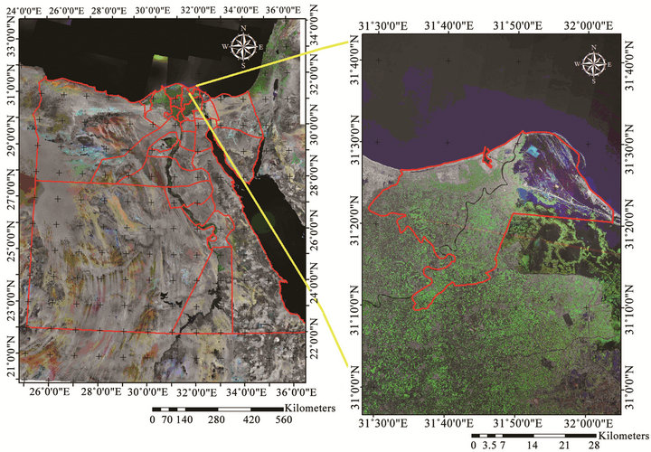
Figure 1. Location of study area (damietta governorate) as false color composition (FCC) of SPOT-4 data.
25˚C in August. The relative humidity is higher in winter than in summer, it attains a minimum average of 68% in May and a maximum average of 76% in August. The evaporation ranges between 2.8 mm/day in December and January and 5.4 mm day in June. Most of the rain falls during November-February; summer is virtually dry. The maximum amount (25.5 ram) is received during winter either in December and/or January. During August and September trace rainfall occurred. According to the keys to soil taxonomy [19], the soil temperature regime of the studied area is defined as Thermic and soil moisture regime as Torric. Two main landscapes can be identified in Damietta Governorate: 1) the coastal plain, adjacent to the Mediterranean, and 2) The flood plain occurring along Damietta Nile branch and El-Dakhalia Governorate. A wide interference zone of fluvio-marine origin lies in between. The coastal plain contains many landforms such as sand beaches, low laying shore ridges, sand sheets, man made terraces, evaporation basins, longitudinal and Barchan sand dunes, hummocks, terraces and overflow and decantation basins, in addition to small areas representing another landforms such as depressions, submerged swamps, and water bodies. The flood plain includes over flow basins, decantation basins, river terraces and levees.
The soil texture of Damietta Governorate differs from place to another due to the alternative pattern of sedimentation and their sediments originated from different parent materials like fluvio-marine deposits, marine deposits, marine aeloian deposits and alluvial deposits. Where soil of the coastal plain along the coast line is sandy, soil texture in the fluvio-marine transitional zone is affected mainly by both the sea and the river Nile showing medium to heavy texture. Texture of the flood plain soils is nearly similar to the texture of the fluviomarine soils (medium to heavy textured). The soils classified to Typic psammaquents, Typic Torripsamments, and Typic Aquisalids in coastal plain and Soils of fluviomarine deposits are Typic Torrifluvents, Typic Fluvequnts, Sodic Psammaqunts and Typic Torripsamments while soils of Alluvial plain are Vertic Torrifluvents and Typic Torrifluvents.
3. Materials and Methods
The methodology of this work focused on field hyperspectral measurements and statistical analysis for the output measurements in order to choose the optimal spectral zone to isolate each crop and then to choose the optimal waveband/s inside each spectral zone that can be used to isolate each crop. As the final objective of this work is presenting information that could be used to increase the accuracy and performance of the existing remote sensing software’s in classifying the different crops in the intensive cultivated lands of the Nile delta. The study compared two summer crops that are cultivated at the same time and again compared the two winter crops. The full description of the used methodology is explained in the following sub-sections.
3.1. Field Hyper Spectral Measurements
Analytical field spectroradiometer (ASD Field Spec) was used to measure the reflection of the four crops under investigation. Wheat and clover measurements were carried out during winter season while rice and maize measurements were carried out in summer season. The average of thirty points distributed along the study area for each crop was calculated to be used in the study. Measurements were carried out in a full optical spectral range (Visible - Near Infrared - Short Wave Infrared) starting from 350 nm to 2500 nm with 1 nm interval output data. The sampling interval is 1.4 nm at the spectral range (350 - 1050 nm) while it is 2 nm at the spectral range (1000 - 2500 nm). These are the intervals which the device is capturing the reflectance. The device automatically performs an interpolation for the data and gives the final data output with (1 nm) interval for the all spectrum range (350 - 2500 nm). The spectrum characteristics of the device are shown in Table 1. The protocol used for the collection of spectral data was based on measuring radiance from a Spectralon® panel. Then, a designed probe was attached to the instrument’s fiber-optic cable was used to ensure standardized environmental conditions for reflectance measurement. The fiber-optic cable provides the flexibility to adapt the instrument to a wide range of applications. The measurements were performed by holding the pistol grip by hand. Bare foreoptic 25 degrees used for outdoor measurements resulting circular field of view with 3 cm diameter as measurements were taken at 3 cm height in nadir position (90 degrees) over the measured plants. As recommended in the instructions of using the device, the Spectralon® was tilted directly towards the sun during optimization.
3.2. One Way ANOVA and Tukey’s HSD Post Hoc Analysis
Spectral zones that represent the atmospheric windows (portions of the electromagnetic reflectance that include
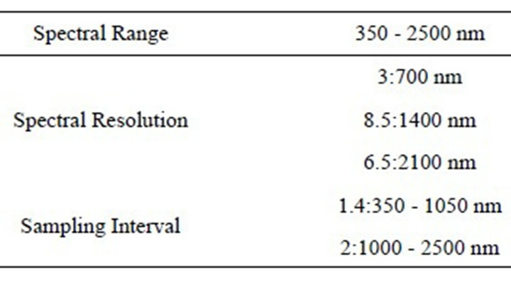
Table 1. The ASD field spec 3 specifications.
data noise because of the relative air humidity) were removed. Spectral pattern of each measured sample was identified. Generally, spectral reflectance could be divided into six different spectral portions as follows: blue (350 - 440 nm), green (450 - 540 nm), red (550 - 750 nm), NIR (760 - 1000 nm), SWIR I (1010 - 1775 nm) and SWIR II (2055 - 2315 nm).
3.2.1. Comparing Standard Deviations from Several Populations
Analysis of variance (ANOVA) methods are presented for comparing means from several populations or processes. While similar methods are occasionally used for comparing several standard deviations, often using the natural logarithm of sample variances as the response variable, they are not a main focal point of this work. There are also a number of alternative procedures that are not based on ANOVA methods that can be used to compare standard deviations. Two of these are described below. Both are highly sensitive to departures from the assumption of normality; consequently, they should be used only after verification that the assumption of normally distributed errors is reasonable. When using ANOVA models with data from designed experiments, a valuable assessment of the assumption of constant standard deviations across k factor-level combinations is given by the Fmax test The Fmax test is used to test the hypotheses [20] (Equation (1)).
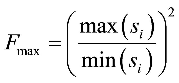 (1)
(1)
3.2.2. Multiple Comparisons
The F-statistics in an ANOVA table provide the primary source of information on statistically significant factor effects. However, after an F-test in an ANOVA table has shown significance, an experiment usually desires to conduct further analyses to determine which pairs or groups of means are significantly different from one another [20].
3.2.3. Tukey’s Significant Difference Procedure
Tukey’s procedure controls the experiment wise error rate for multiple comparisons when all averages are based on the same number of observations. The stated experiment wise error rate is very close to the correct value even when the sample sizes are not equal. The technique is similar to Fisher’s LSD procedure. It differs in that the critical value used in the TSD formula is the upper 100α% point for the difference between the largest and smallest of k averages. This difference is the range of the k averages, and the critical point is obtained from the distribution of the range statistic, not from the t-distribution (Equation (2)).
Two averages  and
and , based on
  and
and  observations respectively, are significantly different if:

where
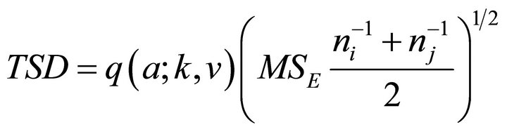 (2)
(2)
3.3. Linear Discriminate Analysis
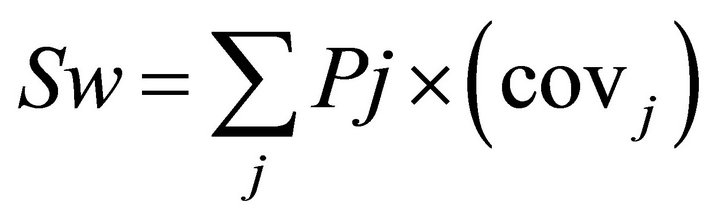
Linear Discriminate Analysis (LDA) is a method to discriminate between two or more groups of samples. The groups to be discriminated can be defined either naturally by the problem under investigation, or by some preceding analysis, such as a cluster analysis. The number of groups is not restricted to two, although the discrimination between two groups is the most common approach. Linear Discrimination Analysis (LDA) is a commonly used technique for data classification. LDA approach is explained by [21]. It easily handles the case where the within-class frequencies are unequal and their performance has been examined on randomly generated test data. This method maximizes the ratio of between-class variance to the within-class variance in any particular data set thereby guaranteeing maximal separability. LDA doesn’t change the location but only tries to provide more class separability and draw a decision region between the given classes. This method also helps to better understand the distribution of the feature data. In the current study, Class-independent transformation type of LDA was performed. This approach involves maximizing the ratio of overall variance to within class variance. It uses only one optimizing criterion to transform the data sets and hence all data points irrespective of their class identity are transformed using this transform. In this type of LDA, each class is considered as a separate class against other classes. In LDA, within-class and betweenclass scatter are used to formulate criteria for class separability. Within-class scatter is the expected covariance of each of the classes. The scatter measures are computed using Equations (3) and (4).
 (3)
(3)
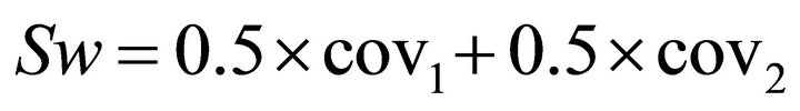
Therefore, for the two-class problem,
 (4)
(4)
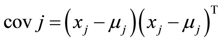
All the covariance matrices are symmetric. Let and be the covariance of set 1 and set 2 respectively. Covariance matrix is computed using the following Equation (5).
 (5)
(5)
Then, the between-class scatter is computes using the following Equation (6).
 (6)
(6)
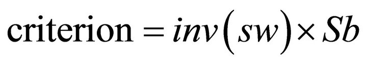
Sb can be thought of as the covariance of data set whose members are the mean vectors of each class. As defined earlier, the optimizing criterion in LDA is the ratio of between-class scatter to the within-class scatter. The solution obtained by maximizing this criterion defines the axes of the transformed space. As LDA is a class independent type in this study, the optimizing criterion is computed as Equation (7)
 (7)
(7)
Finally, transforming the entire data set to one axis provides definite boundaries to classify the data. The decision region in the transformed space is a solid line separating the transformed data sets thus Equation (8)
 (8)
(8)
This analysis was carried out twice to discriminate between wheat and clover and again between maize and rice.
4. Results and Discussion
Spectral reflectance pattern for the four crops is shown in Figure 2. Reflectance pattern showed the same trend for the four crops, however, reflectance of clover and maize was higher than reflectance of wheat and rice along the whole spectrum. The highest spectral reflectance was shown in infrared spectral zone (700 - 1300 nm), relatively low reflectance in the spectral zone (1450 - 1800 nm) while the lowest reflectance was found in the spectral zone (1950 - 2300 nm). It is noticeable that there is a big similarity in the spectral reflectance pattern between rice and wheat. The reason of this might be the close characterization and plant structure of the two crops as they both belong to order: Poales, family: Poaceae. The results of Tukey’s HSD test showed the significancy of the spectral difference between each couple of crops along the six spectral zones attached with the general mean of the reflectance for the two crops, the mean of the reflectance for each crop, the maximum and minmum reflectance values for each crop. The significancy of the difference between the two crops also appears in each figure. Tukey’s HSD test showed that NIR spectral zone is the best to differentiate between wheat and clover followed by SWIR-1 and SWIR-2 that showed relatively high potentiality to differentiate between these two crops. At the same time, visible spectral zones (blue, green and red) did not show significant difference in the reflectance of the two crops as shown in Figure 3; however, blue spectral zone was relatively better than the other two visible spectral zones. Green spectral zone almost did not show any significant spectral reflectance difference be-
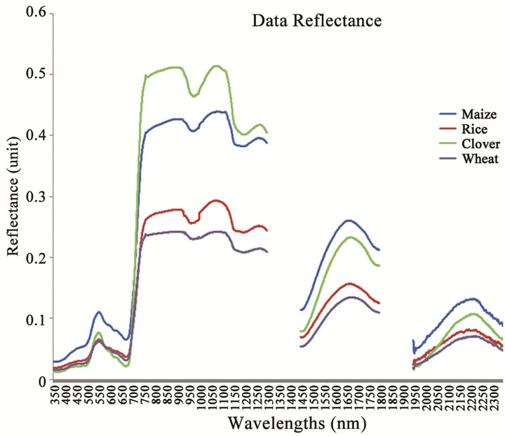
Figure 2. The spectral reflectance pattern for the different crops.
tween wheat and clover.
For the discrimination between rice and maize, the six spectral zones were sufficient to classify the two crops as explained in Figure 4. NIR showed the best result to discriminate between these two crops. The result of the linear discrimination analysis showed the optimal wavebands to differentiate the four crops as shown in Table 2. As shown in this table, only one waveband range in NIR spectral zone was the optimal to isolate maize from rice and to isolate clover from wheat. At the same time, three spectral waveband zones were identified to isolate wheat and rice.
The process of this work included applying two statistical analyses on the spectral measurements of the field spectroradiometer. The main objective was to identify the best spectral zone as the first step and the optimal waveband as the second step to discriminate between the two winter crops (wheat and clover) and the two summer crops (rice and maize). The final objective is to improve the performance of the existing remote sensing software’s in classifying the different crops or other vegetation types through machine learning process. Comparing the spectral reflectance pattern for the two crops showed high spectral similarity between rice and wheat. At the same time, the results showed the clear difference between these two crops and the other two crops (maize and clover). This explains the certainty of spectroradiometric characteristics as a method to differentiate between the different objects. Same method showed high certainty to classify microorganisms as observed by [22]. The results of the statistical analysis explained that NIR spectral zone (700 - 1300 nm) is the best spectral zone to differentiate between each two crops. Only one specific spectral zone, (727:1299 nm in the case of clover and 730:1299 nm in the case of maize), was found the best to

Figure 3. ANOVA and Tukey’s HSD analysis to differentiate between wheat and clover.
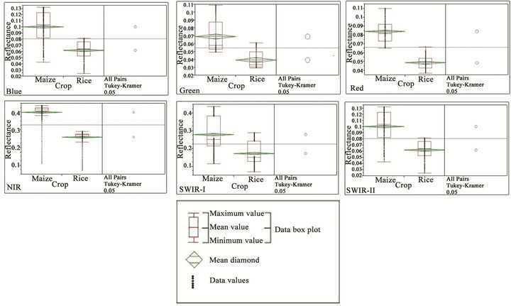
Figure 4. ANOVA and Tukey’s HSD analysis to differentiate between rice and maize.
isolate maize and clover. At the same time, three spectral wavebands were sufficient to isolate wheat (350:712, 1451:1562, 1951:2349 nm) while three spectral wavebands were sufficient to isolate rice 350:713, 1451:1532, 1951:2349 nm). All measurements were carried out during the stage of the maximum vegetative growth for all

Table 2. The optimal waveband to differentiate between the different crops.
crops. The close spectral wavebands that could be used to classify rice and wheat as shown in the results explained that in the case of the classification between closely structure crops, using only the spectral characteristics of the stage of the maximum vegetative growth may not enough and there is a need to assess the spectral characteristics through all growing stages. It could be concluded from the results that vegetation indices that are based on the ratio between NIR, SWIR-I and SWIR-II may be more sufficient to isolate wheat and clover than other indices that are based on visible spectrum. On the other hand, in the case of the differentiation between rice and maize, using vegetation indices that are based on the ratio between NIR and any other spectral zone (visible or invisible) may give adequate results. This work showed the capability of this method to classify crops, however, some modifications in the methodology like multi-temporal measurements during crop growing season may enable the discrimination between very close crops like wheat and barley as an example.
5. Conclusion
Field hyper spectral measurements were used to discriminate between two summer crops (rice and maize) and two winter crops (wheat and clover). Two steps of statistical analysis showed the best spectral zone and the optimal wavebands to discriminate between each two crops. Tukey’s HSD test indicated that NIR spectral zone was the best while green ones were the worst to discriminate between wheat and clover. NIR spectral zone also was the best to discriminate between maize and rice. The other spectral zones showed also acceptable results to differentiate between the same crops. Linear discrimination analysis showed specific wavebands to isolate each crop from the other one. It was found that the wavebands (350:712, 1451:1562, 1951:2349 nm) were the best to isolate wheat while only one waveband (727:1299 nm) was found the best to isolate clover. For the two summer crops, the waveband (730:1299 nm) was the best to isolate maize while three wavebands could be used to isolate rice 350:713, 1451:1532, 1951:2349 nm). Spectral field measurements were carried out for thirty points for each crop distributed along the study area during the maximum vegetative growth of the crops and the average of each crop was considered for the statistical process. Comparing the spectral reflectance pattern for the four crops showed high similarity between rice and wheat.
REFERENCES
- J. R. Anderson, E. T. Hardy, J. T. Rocha and R. E. Witmer, “Land Use and Land Cover Classification System for Use with Remote Sensor Data,” US Geological Survey Professional Paper, Government Printing Office, Washington DC, 1976.
- R. J. Kauth and G. S. Thomas, “The Tasselled Cap—A Graphic Description of the Spectral Temporal Development of the Agricultural Crops as Seen by Landsat,” In: Proceedings of the Symposium on Machine Processing of Remotely Sensed Data, Purdue University, West Lafayette, 2004, pp. 4B-41-4B-51.
- S. G. Wheeler and P. N. Misra, “Linear Dimensionality of Landsat Agricultural Data with Implications for Classifications,” In: Proceedings of the Symposium on Machine Processing of Remotely Sensed Data, Laboratory for Applications of Remote Sensing, West Lafayette, 1976, pp. 2A-1-2A-9.
- E. P. Crist and R. J. Kauth, “The Tasseled Cap De-Mystified,” Photogrammetric Engineering and Remote Sensing, Vol. 52, No. 1, 1986, pp. 81-86.
- G. M. Foody, “Estimation of Land Coverage from Land Cover Classification Derived from Remotely Sensed Data,” GeoJournal, Vol. 36, No. 4, 1995, pp. 361-370. doi:10.1007/BF00807952
- M. L. Nirala and G. Venkatachalam, “Rotational Transformation of Remotely Sensed Data for Land Use Classification,” International Journal of Remote Sensing, Vol. 21, No. 11, 2000, pp. 2185-2202. doi:10.1080/01431160050029503
- H. N. S. Prakash, P. Nagabhushan and G. K. Chidanada, “Symbolic Agglomerative Clustering for Quantitative Analysis of Remotely Sensed Data,” International Journal of Remote Sensing, Vol. 21, No. 17, 2000, pp. 3239- 3251. doi:10.1080/014311600750019868
- Z. Su, “Remote Sensing of Land Use and Vegetation for Mesoscale Hydrological Studies,” International Journal of Remote Sensing, Vol. 21, No. 2, 2000, pp. 213-233. doi:10.1080/014311600210803
- J. E. Vogelmann, T. Sohl and S. M. Howards, “Regional Characterization of Land Cover Using Multiple Sources of Data,” Photogrammetric Engineering and Remote Sensing, Vol. 61, No. 1, 1998, pp. 45-57.
- C. Homer, C. Yuang, Y. Limain, Y. B. Wylie and M. Coan, “Development of a 2001 National Land Cover Database for the United States,” Photogrammetric Engineering and Remote Sensing, Vol. 70, No. 7, 2004, pp. 829-840.
- T. M. Lillesand, R. W. Kiefer and J. W. Chipman, “Remote Sensing and Image Interpretation,” 5th Edition, John Wiley and Sons, New York, 2004.
- P. M. Mather, “Computer Processing of Remotely-Sensed Images: An Introduction,” 3rd Edition, John Wiley & Sons, Chichester, 2004.
- M. Kneubuehler, M. E. Schaepman and T. W. Kellenbergerm, “Comparison of Different Approaches of Selecting Endmembers to Classify Agricultural Land by Means of Hyperspectral Data (DAIS7915),” IEEE International Geoscience and Remote Sensing Symposium Proceedings, Seattle, 6-10 July 1998, pp. 888-890.
- P. S. Thenkabail, E. A. Enclona, M. S. Ashton and B. Van Der Meer, “Accuracy Assessments of Hyperspectral Waveband Performance for Vegetation Analysis Applications,” Remote Sensing of Environment, Vol. 91, No. 3-4, 2004, pp. 354-376.
- G. A. Blackburn, “Quantifying Chlorophylls and Caroteniods at Leaf and Canopy Scales: An Evaluation of Some Hyperspectral Approaches,” Remote Sensing of Environment, Vol. 66, No. 3, 1998, pp. 273-285. doi:10.1016/S0034-4257(98)00059-5
- G. A. Carter, “Reflectance Bands and Indices for Remote Estimation of Photosynthesis and Stomatal Conductance in Pine Canopies,” Remote Sensing of Environment, Vol. 63, No. 1, 1998, pp. 61-72. doi:10.1016/S0034-4257(97)00110-7
- M. Shibayama and T. Akiyama, “Estimating Grain Yield of Maturing Rice Canopies Using High Spectral Resolution Resenescence Flectance Measurements,” Remote Sensing of Environment, Vol. 36, No. 1, 1991, pp. 45-53. doi:10.1016/0034-4257(91)90029-6
- P. J. Curran, J. L. Dungan and H. L. Gholz, “Exploring the Relationship between Reflectance Red Edge and Chlorophyll Content in Slash Pine,” Tree Physiology, Vol. 7, No. 1-4, 1990, pp. 33-48. doi:10.1093/treephys/7.1-2-3-4.33
- USDA, “Keys to Soil Taxonomy,” 11th Edition, United States Department of Agriculture, Natural Resources Conservation Service (NRCS), New York, 2010.
- R. L. Mason, R. F. Gunst and J. L. Hess, “Statistical Design and Analysis of Experiments with Applications to Engineering and Science,” 2nd Edition, John Wiley & Sons, Hoboken, 2003.
- S. Axler, “Linear Algebra Done Right,” Springer-Verlag New York Inc., New York, 1995.
- M.A. Aboelghar and H. A. Abdel Wahab, “Spectral Footprint of Botrytis cinerea, a Novel Way for Fungal Characterization,” Advances in Bioscience and Biotechnology, Vol. 4, No. 3, 2013, pp. 374-382. doi:10.4236/abb.2013.43050