American Journal of Climate Change
Vol. 2 No. 2 (2013) , Article ID: 33501 , 12 pages DOI:10.4236/ajcc.2013.22012
Three Dimensional Numerical Modeling of Flow and Pollutant Transport in a Flooding Area of 2008 US Midwest Flood
National Center for Computational Hydroscience and Engineering, The University of Mississippi, Oxford, USA
Email: *chao@ncche.olemiss.edu
Copyright © 2013 Xiaobo Chao et al. This is an open access article distributed under the Creative Commons Attribution License, which permits unrestricted use, distribution, and reproduction in any medium, provided the original work is properly cited.
Received January 23, 2013; revised February 25, 2013; accepted March 7, 2013
Keywords: 3D Numerical Model; Wind-Driven Flow; Pollutant Transport; Satellite Imagery; US Midwest Flood
ABSTRACT
This paper presents the development and application of a three-dimensional numerical model for simulating the flow field and pollutant transport in a flood zone near the confluence of the Mississippi River and Iowa River during the US Midwest Flood in 2008. Due to a prolonged precipitation event, a levee along the Iowa River just upstream of Oakville, Iowa broke, and the small town was completely flooded for a couple of weeks. During this period, the high water level in the flood zone reached about 2.5 meters above the ground, and wind was the major force for the flow circulation. It was observed that some pollutants were leaked from the residential and farming facilities and transported into the flood zone. Leaking of pollutants from these facilities was reported by different news media during the flood and was identified using high resolution satellite imagery. The developed 3D numerical model was first validated using experimental measurements, and then applied to the flood inundated zone in Oakville for simulating the unsteady hydrodynamics and pollutant transport. The simulated pollutant distributions were generally in good agreement with the observed data obtained from satellite imagery.
1. Introduction
The Midwestern United States is one of four US geographic regions, consisting of 12 states in the United States: Illinois, Indiana, Iowa, Kansas, Michigan, Minnesota, Missouri, Nebraska, North Dakota, Ohio, South Dakota, and Wisconsin. This region has a long history of flooding, with major floods occurring several times over the recent century including 1927, 1961, 1993, 2008, and 2011. Minor flooding is a regular occurrence.
Due to a long term precipitation from December 2007 to June 2008, the Midwest had experienced one of the most wettest winter and spring, causing the soil to become so saturated that additional rainfall could quickly became runoff. In June 2008, much of the Midwestern portions received over 300 mm of rainfall as several storm systems sequentially impacted the region. The vast majority of the precipitation across the region was channeled directly into the lakes, rivers, and streams as runoff, resulting in stream flows reaching historic heights across the Midwest, particularly in many areas of Iowa, southern Wisconsin, and northern Illinois [1,2].
Huge flooding events were reported along the Mississippi River and its tributaries. A number of rivers overflowed for several weeks at a time and levees breached in numerous locations. Historical record high stream flows occurred in some of the major regional rivers including the Des Moines, Cedar and Wisconsin Rivers. Reported river crests exceeded 500-year levels in some locations. It was reported that about twenty-two levees were breached forcing evacuations and causing extensive damage by June 20, 2008. Several states, including Illinois, Indiana, Iowa, Michigan, Minnesota, Missouri, and Wisconsin, were affected by the flooding events. Navigation along the Mississippi River was affected with several of the lock and dam structures closed. The flood left two dozen people killed, 148 injured, approximately 35,000 - 40,000 people evacuated from homes and the damage region-wide was estimated to be in the tens of billions of dollars [1].
A levee of the Iowa River near Mississippi River failed in the evening of June 14, and the water in Iowa River completely flooded the town of Oakville, and thousands of acres of farmland were under water. Since the flooded water was controlled by the levees of Iowa River, Mississippi River, and a hilly area of the Mississippi Valley, an inundation zone was formed for several weeks [3,4]. As there was no outlet, after the water rose to the highest level, it kept for several days. It was observed that some pollutants, such as sewage, pig farm waste, diesel fuel and farm chemicals were leaked and transported in the water [5]. To study the transportation of the pollutant, the inundation zone was treated as a natural lake.
Due to the lack of field measured data, numerical modeling is one of the most effective approaches to study the pollutant transport processes in the flooding zone. Some well-established models, such as ECOMSED developed by Hydroqual, EFDC and WASP developed by the US Environmental Protection Agency (USEPA), CEQUAL-ICM developed by the US Army Corp of Engineers (USACE), have been used by many researchers to study the flow, water quality and pollutant transport in natural water bodies [6-9]. Dortch et al. [10] applied the CH3D-WES hydrodynamic model, originally developed by USACE, to simulate the flow field and pollutant transport of Lake Pontchartrain due to the large amount of contaminated floodwater induced by Hurricane Katrina being pumped into the lake.
A three dimensional numerical model, CCHE3D, has been developed by the National Center for Computational Hydroscience and Engineering (NCCHE) to simulate the flow and sediment transport in natural water bodies [11]. In this study, a 3D model was developed based on CCHE3D to simulate the flow fields and pollutant transport in the Oakville flood inundation zone. After the flooding wave propagation due to the levee breaching, water level rose to the highest position. The water movement in the inundation zone was mainly driven by the wind and the wind-induced flow was the major force for the pollutant transport. This study presents the validation and application of a 3D numerical model for simulating the wind-driven flow and associated pollutant transport in the flooding area of Oakville during the Midwest Flood. Remote sensing techniques using different satellite imagery acquired during the flood event were used to provide some important information, including topography of study area, locations and dimensions of building and farming facilities, and traces of pollutants on the water surface, etc., for the model’s inputs and validation.
2. Model Description
CCHE3D is a finite-element-based unsteady three-dimensional (3D) free surface turbulence model that can be used to simulate turbulent flows with irregular boundaries and free surfaces. This model is based on the 3D Reynolds-averaged Navier-Stokes equations. By applying the Boussinesq assumption, the turbulent stresses are approximated by the eddy viscosity and the strains of the flow. There are several turbulence closure schemes available including: parabolic eddy viscosity model, mixing length model, k-e model and nonlinear k-e model. This model has been verified against analytical methods and experimental data representing a range of hydrodynamics phenomena [11].
To study the wind-driven flow in the Oakville inundation zone, a parabolic vertical distribution of eddy viscosity was specified to analyze the wind-induced flow. A mass transport model was developed based on CCHE3D hydrodynamic model. The pollutant transport equation was solved using finite element method which was consistent with the numerical method employed in the CCHE3D model.
2.1. Governing Equations
The governing equations of continuity and momentum of the three-dimensional unsteady hydrodynamic model can be written as follows:
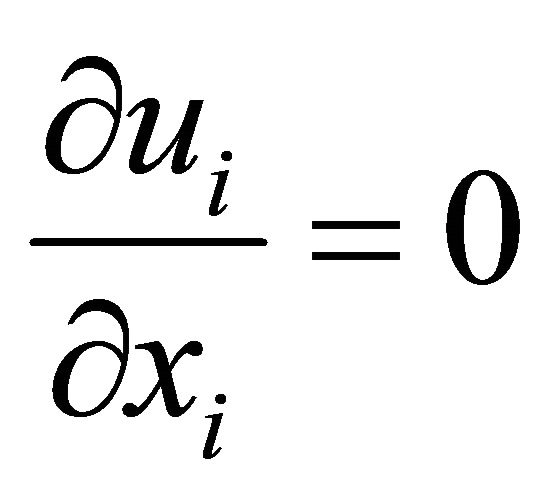 (1)
(1)
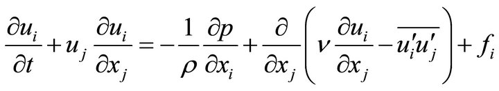 (2)
(2)
where ui (i = 1, 2, 3) are the Reynolds-averaged flow velocities (u, v, w) in Cartesian coordinate system (x, y, z); t is the time; r is the water density; p is the pressure; n is the fluid kinematic viscosity; 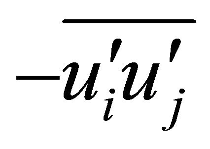 is the Reynolds stress; and fi are the body force terms.
The turbulence Reynolds stresses in Equation (2) are approximated according to the Bousinesq’s assumption. These stresses are related to the mean velocity gradients and the eddy viscosity coefficients. The horizontal eddy viscosity coefficient is computed using the Smagorinsky scheme [12]:
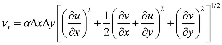 (3)
(3)
where Dx and Dy are the grid lengths in x and y directions, respectively. The parameter a ranges from 0.01 to 0.5.
For wind-driven flow, the vertical eddy viscosity is mainly determined by the wind stresses. Several formulas were presented to calculate the wind-induced eddy viscosity (Section 2.2).
The free surface elevation (hs) is computed using the following equation:
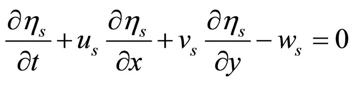 (4)
(4)
where us, vs and ws are the surface velocities in x, y and z directions; hs is the water surface elevation.
The pollutant transport equation can be expressed by:
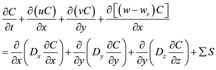 (5)
(5)
in which u, v, w are the water velocity components in x, y and z directions, respectively; ws is the settling/floating velocity; C is the pollutant concentration in water column; Dx, Dy and Dz are the diffusion coefficients in x, y and z directions, respectively;  is the effective source term.
2.2. Wind-Induced Eddy Viscosity
In a natural lake or the Oakville flood inundation zone, wind stress is the important driving force for flow circulation. For simulating the wind driven flow, the distribution of vertical eddy viscosity is required. A parabolic eddy viscosity distribution was proposed by Tsanis [13] based on the assumption of a double logarithmic velocity profile. The eddy viscosity was expressed as:
 (6)
(6)
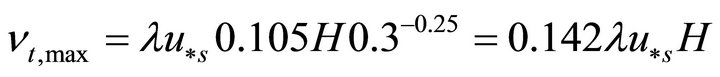
in which l is the numerical parameter; zb and zs are the characteristic lengths determined at bottom and surface, respectively; u*s is the surface shear velocity; H is the water depth. To use this formula, three parameters, l, zb and zs have to be specified. For some real cases with very small water depths, it may cause some problems using this formula to calculate eddy viscosity.
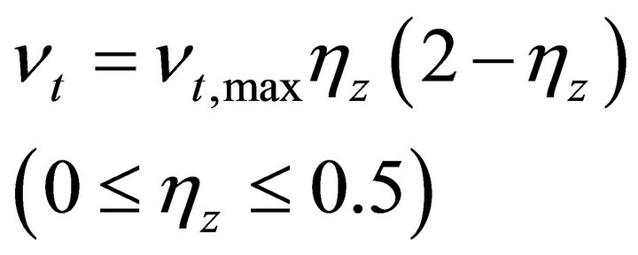
Koutitas and O’Connor [14] proposed two formulas to calculate the eddy viscosity based on a one-equation turbulence model. Their formulas were:
 (7)
(7)
 (8)
(8)
where
 (9)
(9)
in which, l is the numerical parameter; hz is the nondimensional elevation,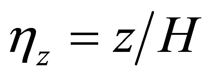 .
.
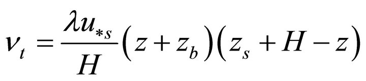
In this study, a new formula was proposed to calculate the wind-induced eddy viscosity based on experimental measurements conducted in a laboratory flume with steady-state wind driven flow reported by Koutitas and O’Connor [14]. The vertical distribution of eddy viscosity was measured and used to fit a calculation formula.
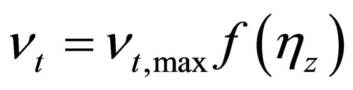
In the proposed formula, the form of eddy viscosity was similar to Koutitas and O’Connor’s assumption (Equations (7) and (8)) and expressed as:
 (10)
(10)
Based on measured data, a formula was obtained to calculate the vertical eddy viscosity:
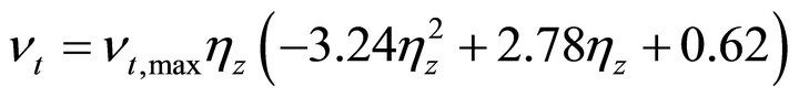 (11)
(11)
Figure 1 compares the vertical distributions of eddy viscosity obtained from experimental measurements and formulas provided by Tsanis (Equation (6)), Koutitas (Equations (7) and (8)), and the proposed formula (Equation (11)). The proposed formula can be used to calculate the eddy viscosity over the full range of water depth. At water surface ( ), Equations (6) and (8) show the eddy viscosity is zero or very closed to zero. The newly proposed formula shows due to the effect of wind shear, the eddy viscosity at the water surface is about 16% of the maximum eddy viscosity
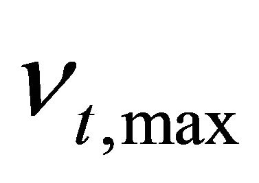 . This formula was used to calculate the vertical eddy viscosity in this study.
2.3. Boundary Conditions
Wind stress is generally the dominant driving force for flow currents in natural lakes. The wind shear stresses at the free surface are expressed by
![]() (12)
(12)
![]() (13)
(13)
where  is the air density; Uwind and Vwind are the wind velocity components at 10 m elevation in x and y directions, respectively. Although the drag coefficient Cd may vary with wind speed [14,15], for simplicity, many researchers assumed the drag coefficient was a constant on
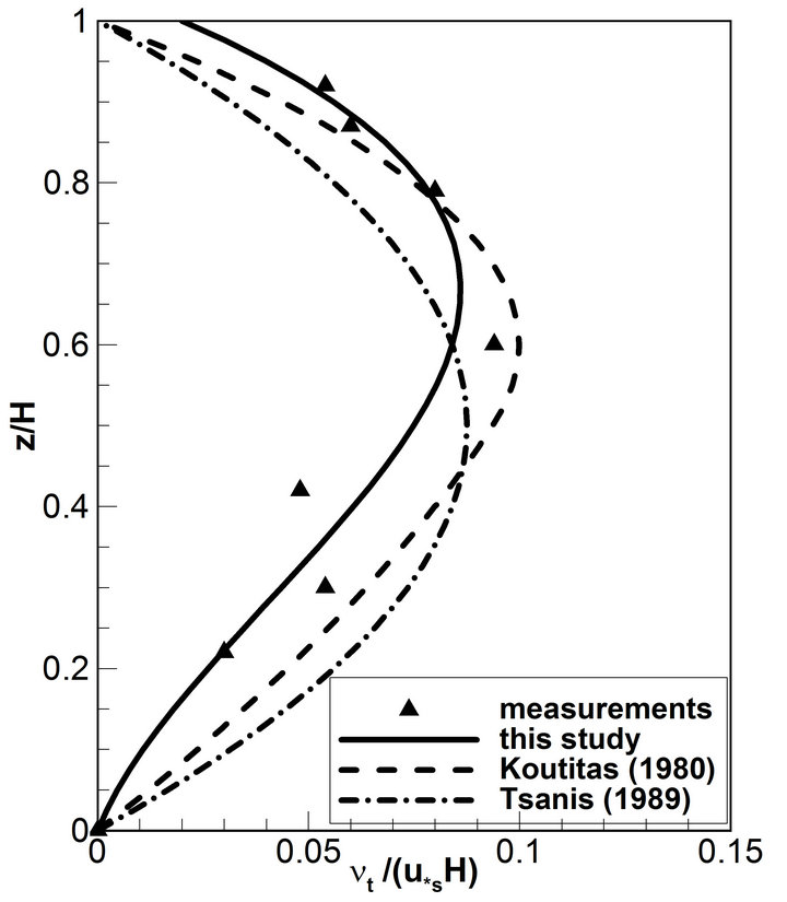
Figure 1. Comparison of vertical eddy viscosity formulas and experimental data.
the order of 10−3 [16,17]. In this model, Cd was set to 0.001, and this value is applicable for simulating the wind driven flow in several natural lakes [18,19].
On the free surface, the normal gradient of pollutant concentration was set to be equal to zero. In the vicinity of the solid walls and bed, the gradients of flow properties were steep due to wall effects. The normal gradient of concentration on the wall was set to be zero.
There are many dry areas in the flooded zone, which represent the buildings of farmer facilities and islands, and wet and dry technique was applied to those areas. In the model, non-slip and the zero normal gradients boundary conditions were set for simulating the flow velocity and pollutant concentration, respectively.
2.4. Numerical Solution
The numerical model was developed based on the finite element method. Each element is a hexahedral with three levels of nine-node quadrilaterals, and the governing equations are discretized using a 27-node hexahedral (Figure 2).
Staggered grid is adopted in the model. The grid system in the horizontal plane is a structured conformal mesh generated on the boundary of the computational domain. In vertical direction, either uniform or non-uniform mesh lines are employed. In order to get more accurate results, the non-uniform mesh lines are placed with finer resolution near the wall, bed and free surface.
The unsteady equations are solved using the time marching scheme. A second-order upwinding scheme is adopted to eliminate oscillations due to advection. In this model, a convective interpolation function is used for this purpose. This function is obtained by solving a linear and steady convection-diffusion equation analytically over a one-dimensional local element shown in Figure 2. Although there are several other upwinding schemes, such as the first order upwinding, the second order upwinding and Quick scheme, the convective interpolation function is selected in this model due to its simplicity for the implicit time marching scheme [11].
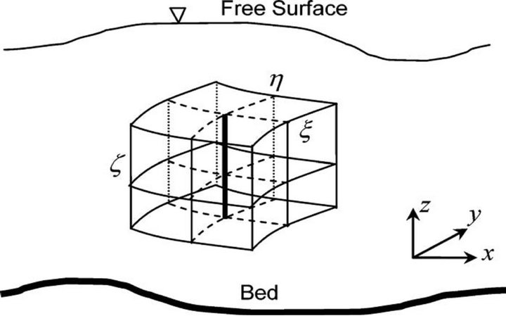
Figure 2. Coordinate system and computational element (in the figure, x , h and z are axes of a local system).
The velocity correction method is applied to solve the dynamic pressure and enforce mass conservation. Provisional velocities are solved first without the pressure term, and the final solution of the velocity is obtained by correcting the provisional velocities with the pressure solution [11]. The system of the algebraic equations is solved using the Strongly Implicit Procedure (SIP) method.
Flow fields, including water elevation, horizontal and vertical velocity components, and eddy viscosity parameters were computed by CCHE3D. After getting the effective source terms SS, the pollutant concentration distribution can be simulated by solving pollutant transport Equation (5) numerically.
3. Model Validation and Verification
3.1. Model Validation for Wind-Driven Flow
A laboratory test case was carried out in a wind-wave flume by Koutitas and O’Connor [14] to study the winddriven flow. The length and width of the measuring flume were 5 m and 0.2 m, and the water depth was 0.31 m. The vertical current profile near the middle section was measured. The developed numerical model was applied to simulate the velocity profile of the wind driven flow for the experimental case. A non-uniform grid with 21 vertical nodes with fine resolution near surface and bed were used for model validation. In the numerical modeling, both Equations (6) and (11) were used for calculating the eddy viscosity, and the simulated vertical velocity profiles were compared with experimental measurements (Figure 3). Numerical results are generally in good agreement with experimental measurements. Near the water surface, the model underestimated the velocity using Tsanis’s formula (Equation (6)) to calculate the eddy viscosity; while it overestimated the velocity by us-
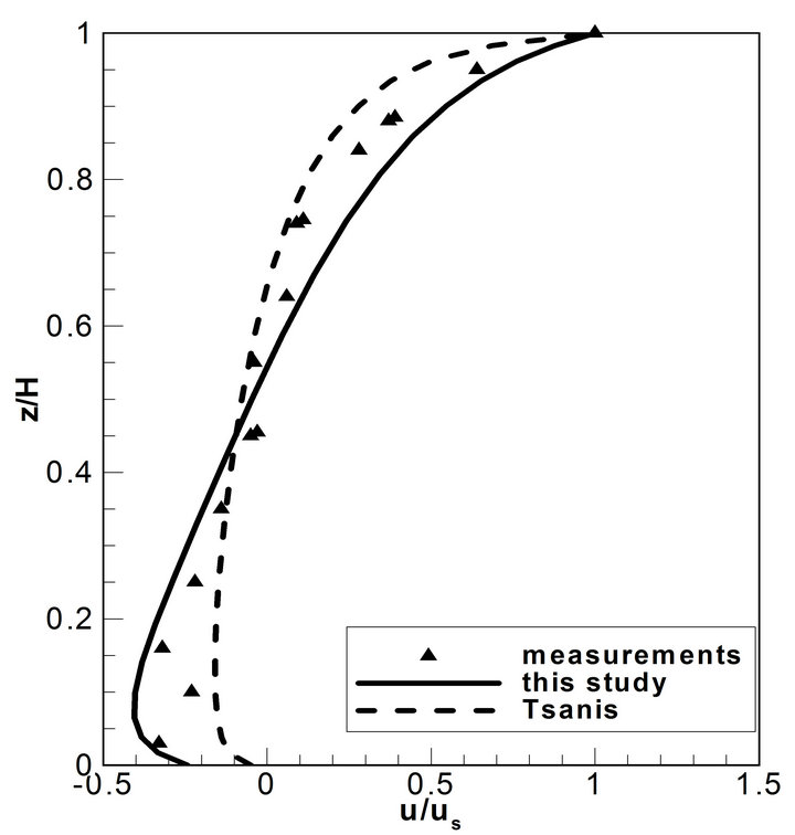
Figure 3. Normalized vertical velocity profile (us = surface velocity).
ing the proposed formula (Equation (11)). Near the bottom, the simulation obtained by using the proposed formula gave better predictions.
3.2. Model Verification for the Mass Transport
The proposed numerical model was tested against an analytical solution for predicting the concentrations of a non-conservative substance in a hypothetical one-dimensional river flow with constant depth and velocity. At the middle of the river, there is a point source with constant concentration (Figure 4). Under this condition, the concentration of the substance throughout the river can be expressed as:
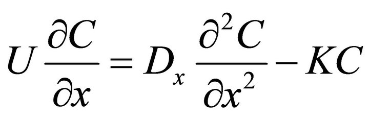 (14)
(14)
where U is the velocity; C is the substance concentration; Dx is the dispersion coefficient; x is the displacement from point O; and K is the decay rate. An analytical solution given by Thomann and Mueller [20] is:
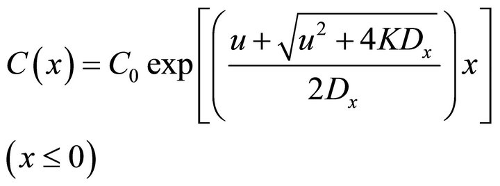 (15)
(15)
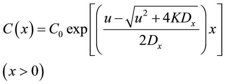 (16)
(16)
where C0 is the concentration at O point. In this test case, it was assumed, the water depth is 10 m and Dx is 30 m2/s, the values of K are 0, 1.0/day and 2.0/day, respectively, Figure 5 shows the concentration distributions obtained by the numerical model and analytical solution. The maximum error between the numerical result and analytical solution is less than 2%.
4. Application to Oakville Flood Zone Due to 2008 US Midwest Flood
4.1. Study Area
Due to a long period of heavy precipitation, a 500-year flood occurred in June 2008 and affected portions of the Midwest United States. In the evening of June 14, a levee
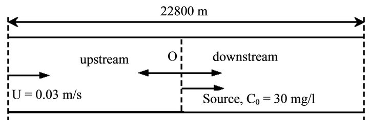
Figure 4. Test river for model verification.
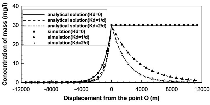
Figure 5. Concentration distribution of non-conservative substance in the test river.
along the Iowa River just upstream of Oakville failed, and the water in the river rushed through the broken levee and completely flooded the small town. Figure 6 shows the flood zone and the location of the levee breaching. As the flooding area was governed by river levees and hilly area, an inundation area was formed and the high water level in this zone tented to remain for several weeks. It was reported that the length of the damaged levee was about 1100 m, and it was not completely fixed until July 1 [2,3,21]. It was estimated from the high water mark, the high water level was about 2.5 meter above the ground [22,23]. It was also observed that some oily pollutants were leaked and transported on the water surface [5]. To study the pollutant transport in the inundation zone, this flooding area can be treated as a natural lake. As this area is relatively flat, the wind is the major driving force of the water flow. To demonstrate the capabilities of the developed model, it was applied to simulate the wind-induced flow and pollutant transport.
Figure 7 shows the computational domain and topography obtained from 30 m resolution of USGS Digital Elevation Model (DEM). The inundation zone was an enclosed water body with the north-south axis spanning about 16 km, while the shorter east-west axis was about 8 km. There were many residential houses and farm facilities in this flooding zone, which could affect the flow fields. In the numerical model, they were represented with a number of dry nodes. The computational mesh was generated using the CCHE Mesh Generator. In the horizontal plane, the computational domain was represented by a 199 × 300 irregular quadrilateral mesh. In the vertical direction, it was divided into 8 non-uniform layers and mesh lines conformed to the curved and irregular bed bathymetry. The vertical distribution of the non-uniform grid was generated using the flexible and powerful two-direction stretching function with finer spacing near the surface and bottom [24].
4.2. Application of Satellite Imagery for Providing Information for Numerical Model
During the flooding events, it is almost impossible to
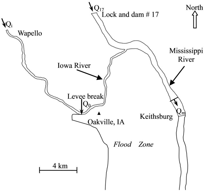
Figure 6. The flood zone and the location of the levee breaching.
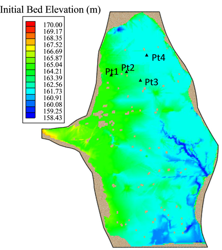
Figure 7. Computational domain.
conduct field measurements to acquire flow field and pollutant distribution data in the inundated areas due to inclement weather conditions. Remote sensing has been widely used as a proven tool to map and monitor flood propagation for many years. During a flood event, nearreal-time satellite imagery serves as a very useful management tool for authorities coping with the disaster [25]. Although the observed data by satellite imagery are limited on the water surface, over the years it has been successfully used for water quality studies. In this studydifferent satellite imagery were acquired, processed and analyzed by digital image processing techniques to generate useful information for model simulation and validation.
A 30 m resolution Landsat 7 ETM+ imagery acquired in 2003 was used to delineate the model domain boundary. A 10 m resolution Advance Land Observing Satellite (ALOS) Advance Visible and Near Infrared Radiometer type 2 (AVNIR2) imagery acquired on June 21, 2008, was used to determine the dimension (length) of the levee failure (Figure 8) and detect and map the locations and sizes of residential houses and farm facilities (Figure 7). This imagery along with another Landsat 5 TM imagery acquired on June 16, 2008 were used to map the traces of pollutants derived by flood water and their nature as well.
Both Landsat and ALOS imagery were visually inspected to map the traces of the pollutants. The imagery was displayed in true color and false color composite with 4 (red), 3 (green), 2 (blue) band combination (Figure 9). Principal Component Analysis (PCA) was performed and image derived spectral profiles were studies to determine the nature of the pollutants [26].
The spectral profiles derived from the visually detected pollutant traces clearly reveals that the pollutants are some kinds of fluid but not water (Figure 10). From the visual inspection it was observed that the pollutants fluenced by winds. The traces were observed on both Landsat and ALOS imagery maintaining the same pattern
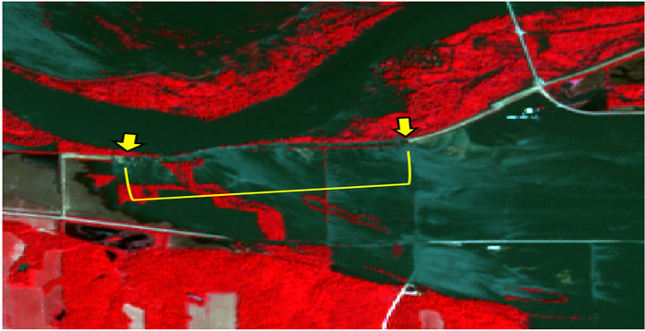
Figure 8. Dimension of levee failure measured (1100 m) on the ALOS AVNIRE 2 imagery acquired on 6/21/2008.
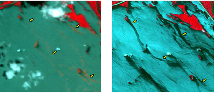
Figure 9. Pollutant traces as observed in satellite imagery during the flood event; Landsat 5 imagery (6/16/2008) ALOS AVNIR 2 imagery (6/21/2008).

Figure 10. Analysis of spectral profiles of pollutants as observed on the ALOS AVNIRE 2 imagery acquired on 6/21/2008.
were floating on the water surface maintaining trails in- (Figure 9). The shape and pattern of these trails clearly indicate that the materials composing the traces were not quickly soluble in the water. By the available satellite data it was not possible to determine the true nature of the pollutant materials since there was no measured data for the pollutants. However, since during the flood event a large amount of gasoline leakage was reported [5], the detected pollutant traces in satellite imagery were considered to be of oily pollutant.
4.3. Flow Simulation
Water flow in the flood zone was primarily wind-driven. Pollutant stripes on the water surface were observed from satellite image acquired at 16:47 hours, June 21, 2008. Those pollutants were apparently leaked from farming facilities, and floated on the water surface. It was observed that their transports were majorly affected by the wind-induced surface flow velocities. To study the flow field as well as pollutant transport on the water surface, the 3D model is needed. In this study, the developed 3D model was applied to simulate the flow field induced by wind, and the pollutant concentration distributions were simulated by solving Equation (5) numerically.
To run the 3D model, the initial flow fields are needed. CCHE2D model was applied to provide initial flow field conditions, including water surface elevation, velocity, shear stress, eddy viscosity, etc., for the 3D model. The CCHE2D model was developed by NCCHE for simulating two dimensional depth-averaged unsteady flow, sediment transport, flood inundation/propagation, levee breaching and pollutant transport [27,28]. It has been successfully applied to simulate the flood events and flood propagation during the Hurricane Katrina and Midwest flood 2008 [29,30]. In this study, CCHE2D model was used to simulate the processes of flood propagation/
inundation due to the levee breaching along the Iowa River near Oakville, and the computed results were set as initial conditions for the 3D model simulation.
The water discharge that entered the Oakville flood zone can be estimated based on the measured discharges at several stations located along Mississippi River and Iowa River, including Lock and dam #17, Keithsburg, and Wapello stations (shown in Figure 6). The following formula was used to calculate the discharge entering the flood zone (Q0):
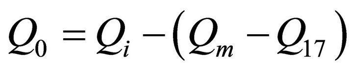 (17)
(17)
where Qi is the flow discharge at Wapello in Iowa River; Qm is the discharge at Keithsburg in Mississippi River; Q17 is the discharge at Lock and dam #17, about 5 km upstream of the confluence of Mississippi River and Iowa River.
Figure 11 shows the discharge that entered the flood zone, causing the water level rising gradually from June 14 to June 24. In CCHE2D model, the discharge was set as inlet boundary for simulating the flood propagation. Figure 12 shows the simulated processes of flood propagation/inundation at different times. It can be found that
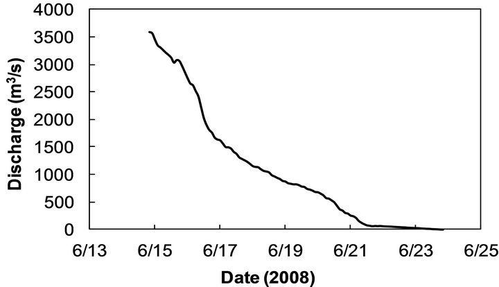
Figure 11. The discharge that entered the Oakville flood zone.
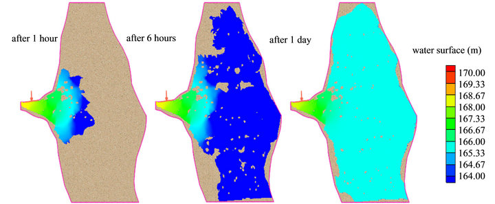
Figure 12. The simulated processes of flood propagation at different times.
almost all the residential houses and farm facilities were inundated within first 6 hours. After one day, the whole area of the tiny town was under the water, and then the water level kept rising until June 21. The simulated results showed that the averaged water depth was about 2.65 m, close to the observed data (2.5 m). The 2D flood simulation results were used as initial conditions for the 3D model flow simulation.
Due to a long period of time submerged under the water, some oily pollutants were leaked from farmer’s facilities and transport in the flooding water. Satellite image (Figure 9) showed that there were some pollutant strips observed on water surface on June 21, 2008. However, one day before, there were no pollutant strips in the same area. It can be estimated that the pollutant leak might occur on June 21. In this study, a period from 6:00 to 18:00 hours, June 21, 2008 was chosen for modeling the flow and pollutant transport in the flooding zone.
Figure 13 shows the observed wind velocities and directions near the study area during the simulation period, and the major wind direction is blowing from northwest, which is consistent with the pollutant moving direction. After obtaining the initial condition provided by the 2D model, the unsteady wind-driven flow fields were simulated using the developed 3D model. Based on some pretests, simulated wind-induced flow fields show similar patterns by using Equations (6) and (11) to calculate the vertical eddy viscosity. In this study, Equation (11) was used to calculate the vertical eddy viscosity in the flood zone.
Figures 14(a) and (b) show the simulated velocity vectors at 4:00 pm on the water surface and near the bottom, respectively. In general, wind-shear forced the flow near the surface to move in the direction of the wind and resulted opposite movement in the lower layers. The water depth and surrounding wall boundaries also affected the circulation of wind driven flow.
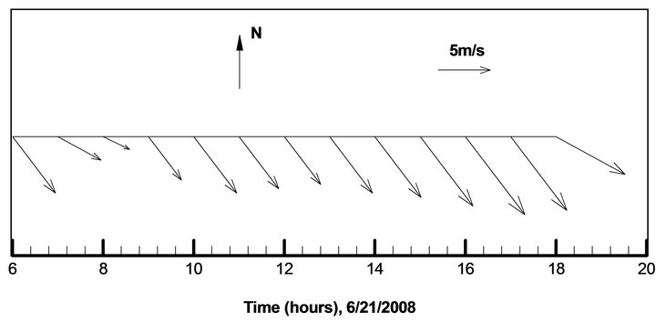
Figure 13. Measured wind speeds and directions (6:00- 18:00 hours, June 21, 2008).
4.4. Pollutant Distribution
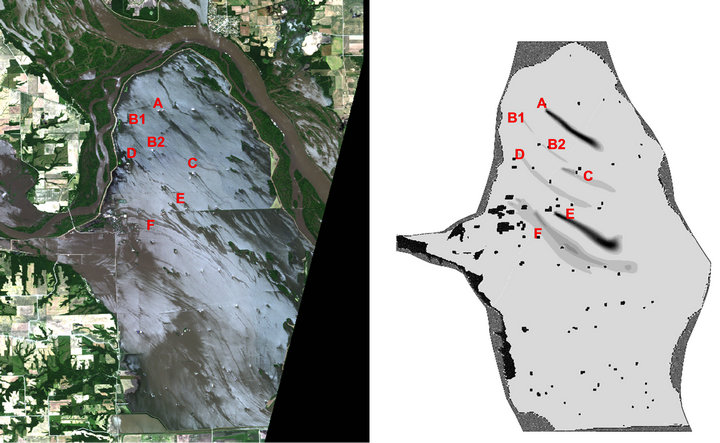
Satellite image showed that the oily pollutants leaked from farming facilities drifted with the flow forming many stripes aligned with the wind and surface flow direction (Figures 9 and 15(a)). After obtaining the simulated flow fields, the 3D model was applied to simulate the oily pollutant transport in this flooding zone. Due to a lack of directly measured data, the amount of pollutants leaking was estimated from the satellite imagery and they were simulated as passive materials. The density of oily pollutant is lighter than water; it may float on the water surface, and move mainly following the water surface velocity.
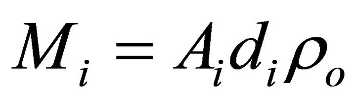
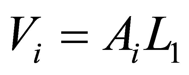
Several locations such as A, B1, B2, C, D, E and F, were selected for simulating the pollutant distribution. In the numerical model, it was assumed that the oily pollutant just moving on the water surface due to the buoyancy force. The leaking rates of the oily pollutant from different locations were set as source terms in Equation (5) and calculated by:
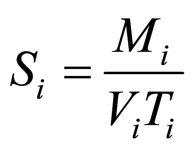 (18)
(18)
in which, Si is the leaking rate of the pollutant at location i; Mi is the total amount of pollutant at location i leaking
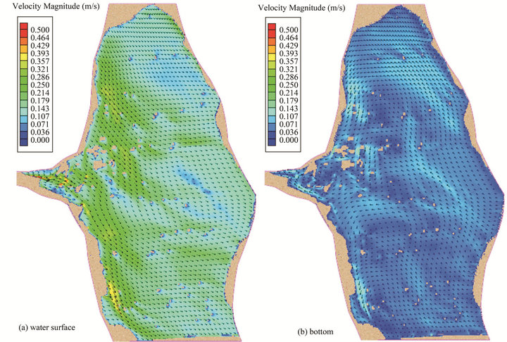
Figure 14. Flow vectors in the flood zone (4:00 pm, 6/21/08).
 (a) (b)
Figure 15. Pollutant distribution in the flood zone (4:47 pm, 6/21/08): (a) Satellite image (10 m resolution ALOS AVNIR 2); (b) Numerical results.
into the water; Ti is the time period for pollutant at location i leaking into the water; and Vi is the volume of surface water layer receiving the pollutant during the Ti time period. The values of Mi , Vi and Ti can be estimated based on the satellite imagery (Section 5).
The simulated pollutant distributions at the locations of A, B1, B2, C, D, E and F were compared with the satellite imaginary (Figures 15(a) and (b)). The main trend of pollution stripes was well predicted. Some differences between the model results and satellite imagery remain due to the uncertainty of occurring time and leaking amount of pollutant. In addition, only one wind station data was available for the simulation and it was applied to the entire flood zone. In reality, wind velocity and direction might change locally over the flood zone.
5. Discussions
5.1. Effect of Vertical Distribution of Computational Mesh on Surface Flow Fields
It was observed that the oily pollutant transports in the flood zone were mainly affected by the wind-induced surface flow velocities. To calculate the wind driven flow, the water body was divided into 8 non-uniform layers vertically with finer spacing near the surface and bottom. The computational meshes with different vertical distributions may produce different surface flow velocity.
In this study, the flow fields computed using 4 meshes with different vertical distributions were compared, and the ratio between the vertical layer depths and the total water depth from top to bottom were listed in Table 1.
In the uniform mesh, the depth of surface layer was 12.5% of the total water depth, which was same as the other layers.
In other three non-uniform meshes, the depths of surface layers were 8%, 6% and 4% of the total depth, respectively. Figure 16 shows the simulated surface velocities at the locations of Pt1, Pt2, Pt3 and Pt4 (Figure 7) using the four meshes with different depths of surface layers. It can be observed that with the decrease of surface depth, the surface velocity increases. The differences of the velocity obtained using Mesh NonUniform2 (L1 = 6%H) and NonUniform3 (L1 = 4%H) were very
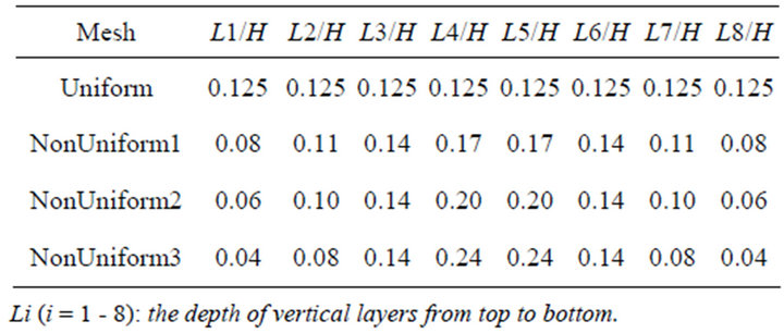
Table 1. The ratio between the vertical layer depth (Li) and the total depth (H) of the four meshes.
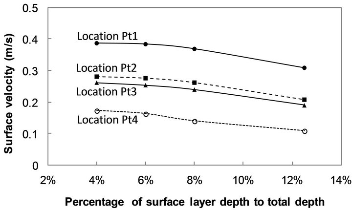
Figure 16. Simulated surface velocities at different locations using four meshes.
small. Therefore, in the study, the Mesh Non-uniform3 was selected for the simulating the flow and pollutant transport in the flood zone.
5.2. Useful Information Obtained from Satellite Imagery for Model Simulation
Due to the lack of direct measured data, it is very challenging work for simulating the flow field and pollutant transport during a flood event. In this study, remote sensing technology was applied to estimate the length of the broken levee, the pollutant leaking period and the pollutant distribution. Based on the pollutant distribution pattern obtained from satellite imagery, it was observed that most of the pollutant shows a strip following the wind direction. Figure 14(a) shows that the wind-induced surface velocity generally follows the wind direction. So the movement of the pollutant is mainly determined by the wind-induced surface flow velocity. This is one of obvious properties of oily pollutant moving on the water surface.
The satellite imagery was also used to estimate the time and location of the pollutant leaking. However, it is quite hard to estimate the amount of pollutant leaking into the flooding water, and the leaking processes. For simplification, the amount of pollutant leaking from each farmer’s facility was estimated based on the polluted area shown on the satellite imagery, and the thickness of the pollutant. Normally, if the thickness of oily pollutant is less than 1 mm, it may be broken [31].
Since the traces of pollutants detected in the satellite imagery did not show any indication of breaking, in this study, the oil pollutant was assumed to be uniformly distributed in the water with 1mm thickness. The polluted area was obtained by mapping the boundary of the oily pollutant in the satellite imagery. The amount of pollutant at location i leaking into the water (Mi) can be estimated by
 (19)
(19)
in which, Ai is the area of polluted area; di is the thickness of oily pollutant (0.001 m); and ro is the density of oily pollutant (~0.9 kg/m3). After obtaining the polluted area, the volume of surface water receiving the pollutant (Vi) in Equation (18) can be calculated by
 (20)
(20)
in which, L1 is the depth of surface water layer. In the model, it was assumed that the pollutant leaking at several locations occurred simultaneously. The satellite image acquired at 16:47 hours, June 21, 2008, the time period Ti in Equation (18) can be simply assumed from the beginning of the pollutant leaking (6:00 am) to 16:47, which is 10 hours and 47 minutes.
6. Summary and Conclusions
A three dimensional model was developed and applied to simulate the wind-driven flow and pollutant transport in natural waters. The model was first validated against measured velocity profile of wind-driven flow obtained in an experimental open channel. Then it was applied to simulate the wind-driven flow and pollutant transport in a flood inundation area in Oakville, IA during the 2008 US Midwest flooding event. The remote sensing technology was used to provide the locations of residential house and farmer’s facility, and the length of the broken levee. It was also used to identify the pollutant distributions in the computational domain and extract pollution source locations.
Based on the field observation and satellite imagery, the pollutants in the studied flood zone were considered as oily material. It was floating on the water surface and mainly driven by the wind-induced surface velocity. The simulation of wind driven flow was tested using several meshes with different vertical uniform and non-uniform distributions, and the mesh with thinner surface and bottom layers (4% of total depth) was selected for the simulating the flow and pollutant transport in the flood zone. The simulated pollutant distributions were generally in good agreement with observations obtained from satellite imagery. This model provides useful information for understanding the flow circulation and pollutant transport in the flooding zone. It may help for developing and implementing an emergency response plan during a flood.
7. Acknowledgements
This research was funded by the US Department of Homeland Security and was sponsored by the Southeast Region Research Initiative (SERRI) at the Department of Energy’s Oak Ridge National Laboratory.
REFERENCES
- National Climatic Data Center, “Climate of 2008 Midwestern US Flood Overview,” 2008. http://www.ncdc.noaa.gov/oa/climate/research/2008/flood08.html
- Federal Emergency Management Agency (FEMA), “Midwest Floods of 2008 in Iowa and Wisconsin,” Report FEMA P-765, October 2009.
- S. M. Linhart and D. A. Eash, “Floods of May 30 to June 15, 2008, in the Iowa River and Cedar River Basins, Eastern Iowa,” US Geological Survey, Open-File Report 2010-1190, Reston, Virginia, 2010.
- Wikipedia, “Iowa Flood of 2008,” 2008. http://en.wikipedia.org/wiki/Iowa_flood_of_2008.
- A. G. Breed, “Flooding: A Greater Disaster Is Yet to Be Felt,” 2008. http://newearthsummit.org/forum/index.php?topic=143.0
- J. A. McCorquodale, I. Georgiou, C. Chilmakuri, M. Martinez and A. J. Englande, “Lake Hydrodynamics and Recreational Activities in the South Shore of Lake Pontchartrain, Louisiana,” Technical Report for NOAA, University of New Orleans, 2005.
- Z. G. Ji, “Hydrodynamics and Water Quality Modelling River, Lakes, and Estuaries,” Wiley-Interscience, Hoboken, 2008. doi:10.1002/9780470241066
- M. R. Ernst and J. Owens, “Development and Application of a WASP Model on a Large Texas Reservoir to Assess Eutrophication Control,” Lake and Reservoir Management, Vol. 25, No. 2, 2009, pp. 136-148. doi:10.1080/07438140902821389
- C. F. Cerco and T. Cole, “User’s Guide to the CE-QUALICM: Three-Dimensional Eutrophication Model,” Technical Report EL-95-15, US Army Corps of Engineers, Vicksburg, 1995.
- M. S. Dortch, M. Zakikhani, S. C. Kim and J. A. Steevens, “Modeling Water and Sediment Contamination of Lake Pontchartrain Following Pump-Out of Hurricane Katrina Floodwater,” Journal of Environmental Management, Vol. 87, No. 3, 2008, pp. 429-442. doi:10.1016/j.jenvman.2007.01.035
- Y. Jia, S. Scott, Y. Xu, S. Huang and S. S. Y. Wang, “Three-Dimensional Numerical Simulation and Analysis of Flows around a Submerged Weir in a Channel Bendway,” Journal of Hydraulic Engineering, Vol. 131, No. 8, 2005, pp. 682-693. doi:10.1061/(ASCE)0733-9429(2005)131:8(682)
- J. Smagorinsky, “Large Eddy Simulation of Complex Engineering and Geophysical Flows,” In: B. Galperin and S. A. Orszag, Eds., Evolution of Physical Oceanography, Cambridge University Press, Cambridge, 1993, pp. 3-36.
- I. K. Tsanis, “Simulation of Wind-Induced Water Currents,” Journal of Hydraulic Engineering, Vol. 115, No. 8, 1989, pp. 1113-1134. doi:10.1061/(ASCE)0733-9429(1989)115:8(1113)
- C. Koutitas and B. O’Connor, “Modeling Three-Dimensional Wind-Induced Flows,” Journal of Hydraulic Engineering, Vol. 106, No. 11, 1980, pp. 1843-1865.
- K. R. Jin, J. H. Hamrick and T. Tisdale, “Application of Three Dimensional Hydrodynamic Model for Lake Okeechobee,” Journal of Hydraulic Engineering, Vol. 126, No. 10, 2000, pp. 758-771. doi:10.1061/(ASCE)0733-9429(2000)126:10(758)
- W. Huang and M. Spaulding, “3D Model of Estuarine Circulation and Water Quality Induced by Surface Discharges,” Journal of Hydraulic Engineering, Vol. 121, No. 4, 1995, pp. 300-311. doi:10.1061/(ASCE)0733-9429(1995)121:4(300)
- F. J. Rueda and S. G. Schladow, “Dynamics of Large Polymictic Lake. II: Numerical Simulations,” Journal of Hydraulic Engineering, Vol. 129, No. 2, 2003, pp. 92- 101. doi:10.1061/(ASCE)0733-9429(2003)129:2(92)
- X. Chao, Y. Jia, F. D. Shields Jr., S. S. Y. Wang and M. C. Charles, “Three-Dimensional Numerical Modeling of Water Quality and Sediment-Associated Processes with Application to a Mississippi Delta Lake,” Journal of Environmental Management, Vol. 91, No. 7, 2010, pp. 1456-1466. doi:10.1016/j.jenvman.2010.02.009
- X. Chao, Y. Jia, S. S. Y. Wang and A. K. M. A. Hossain, “Numerical Modeling of Surface Flow and Transport Phenomena with Applications to Lake Pontchartrain,” Lake and Reservoir Management, Vol. 28, No. 1, 2012, pp. 31-45. doi:10.1080/07438141.2011.639481
- R. V. Thomann and J. A. Mueller, “Principles of Surface Water Quality Modeling and Control,” Harper & Row Publication, New York, 1988.
- R. E. Criss and T. M. Kusky, “Finding the Balance between Floods, Flood Protection, and River Navigation,” Saint Louis University, Center for Environmental Sciences, 2009.
- National Broadcasting Company (NBC) News, “FEMA Flood Maps Are Full of Errors, Cities Say,” January 24, 2010. http://www.msnbc.msn.com/id/35045333/ns/weather/t/fema-flood-maps-are-full-errors-cities-say/#.UOcBwHdtQvw
- National Committee on Levee Safety, “Levee Situation in the US,” 2012. http://www.leveesafety.org/lv_nation.cfm
- Y. Zhang and Y. Jia, “CCHE Mesh Generator and User’s Manual,” Technical Report No. NCCHE-TR-2009-1, University of Mississippi, Oxford, 2009.
- A. K. M. A. Hossain, G. Easson, V. J. Justice and D. Mita, “Mapping Flood Extent, Flood Dynamics, and Crop Damage Assessment Using Radar Imagery Analysis,” MidSouth Annual Engineering & Sciences Conference (MAESC), Oxford Conference Center Oxford, 17-18 May 2007.
- T. M. Lillesand and R. W. Kiefer, “Remote Sensing and Image Interpretation,” 4th Edition, John Willey and Sons, Inc., Hoboken, 2000.
- Y. Jia and S. S. Y. Wang, “Numerical Model for Channel Flow and Morphological Change Studies,” Journal of Hydraulic Engineering, Vol. 125, No. 9, 1999, pp. 924- 933. doi:10.1061/(ASCE)0733-9429(1999)125:9(924)
- Y. Jia, S. S. Y. Wang and Y. Xu, “Validation and Application of a 2D Model to Channels with Complex Geometry,” International Journal of Computational Engineering Science, Vol. 3, No. 1, 2002, pp. 57-71. doi:10.1142/S146587630200054X
- Y. Jia, et al., “Development of an Integrated Simulation Tool for Predicting Disastrous Flooding, Water Contamination, Sediment Transport and their Impacts on the Environment,” Technical Report, Task Order No: 40000647 04, The University of Mississippi, Oxford, 2012.
- Y. Jia, A. K. M. A. Hossain and X. Chao, “Computational Modeling of Midwest Flood 2008: Levee Breaching and Flood Propagation,” ASCE World Environmental and Water Resources Congress, Reston, 2010, pp. 1298-1303.
- X. Chao, N. J. Shankar and S. S. Y. Wang, “Development and Application of a Three-Dimensional Oil Spill Model for Singapore Coastal Waters,” Journal of Hydraulic Engineering, Vol. 129, No. 7, 2003, pp. 495-503. doi:10.1061/(ASCE)0733-9429(2003)129:7(495)
NOTES
*Corresponding author.