American Journal of Industrial and Business Management
Vol. 3 No. 3 (2013) , Article ID: 33728 , 16 pages DOI:10.4236/ajibm.2013.33034
Generalized Demand Densities for Retail Price Investigation
![]()
1School of Engineering and Mathematical Sciences, City University London, London, UK; 2Cass Business School, City University London, London, UK.
Email: pjt3.michaelmas@gmail.com
Copyright © 2013 Philip Thomas, Alec Chrystal. This is an open access article distributed under the Creative Commons Attribution License, which permits unrestricted use, distribution, and reproduction in any medium, provided the original work is properly cited.
Received April 27th, 2013; revised May 30th, 2013; accepted June 28th, 2013
Keywords: Demand Density; Probability Density; Demand Curve; Double Power Demand Density; Rectangular Demand Density; Kinked Demand Density
ABSTRACT
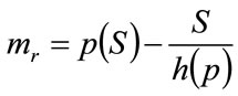
The paper introduces generalized demand densities as a new and effective way of conceptualizing and analyzing retail demand. The demand density is demonstrated to contain the same information as the demand curve conventionally used in economic studies of consumer demand, but the fact that it is a probability density sets bounds on its possible behavior, a feature that may be exploited to allow near-exhaustive testing of possible demand scenarios using candidate demand densities. Four such demand densities are examined in detail. The Household Income demand density is based on the assumption that a person’s maximum acceptable price (MAP) for an item is proportional to his household after-tax income. The Double Power demand density allows the mode to be located anywhere in the range between zero and the highest MAP possessed by anyone in the target population. The two-parameter, Rectangular demand density, the simplest model that a retailer may employ, has the useful feature that it may be matched relatively easily to any unimodal demand density and hence may act as its approximate proxy. The Kinked demand density is derived from the kinked demand curve sometimes used as a relatively uncomplicated way of conceptualizing the effects of oligopoly. The central measures of each of these demand densities are derived: mean price, mode, median, optimal and, when appropriate, the mean of the matched Rectangular demand density. In a further result arising from the use of demand densities, it is shown that stable trading at the kink price will not occur if the demand curve is kinked and convex.
1. Introduction
While a demand curve may be used to investigate retail prices and how they are set [1-3], it has been demonstrated [4] that there are advantages in recasting the information into a probability density for maximum acceptable price (MAP) or “demand density”. The “demand density” allows investigations of the optimal price to proceed in a natural and convenient way. The fundamental restriction on any probability density, namely that its integral over all values must equal unity, turns out to be a particularly useful feature, making the demand density a feasible tool for exploring situations where data are sparse. Here a finite number of demand densities may be employed to provide a near-exhaustive coverage of possible price preferences.
The paper will begin by explaining the equivalence between the demand density curve and the demand curve conventionally shown in economics textbooks. It will show how the price optimization procedure based on demand density produces the same answer as the graphical method based on the demand curve. Having established this equivalence, the paper will go on to consider four demand densities that have been found useful in assessing how retail prices may be set, deriving key properties of
• the Household Income demand density, where MAP is proportional to household income after tax.
• the Double Power demand density, where an appropriate choice of the four defining coefficients allows the mode to be located anywhere in the range between zero and the highest MAP possessed by anyone in the target population.
• the two-parameter, Rectangular demand density, which is the simplest model that a retailer may employ, based on his knowledge only of the lowest price at which he is prepared to sell and the highest price he believes he could charge before sales become negligible.
• the Kinked demand density, derived from the kinked demand curve introduced independently by both Hall and Hitch [5] and Sweezy [6] as a relatively simple way of conceptualizing the effects of oligopoly.
The clear perspective on the optimization procedure promoted by the use of the demand density rather than the demand curve has allowed the correction of a misapprehension concerning the kinked demand curve. The location of the optimal price when that curve is convex is found not to be located at the kink price.
The usefulness of the demand density as a model for retail demand has been found previously not to be greatly compromised when the underlying probability density for MAP is approximated by a Rectangular demand density [4]. Therefore an analytical procedure will be presented that allows a Rectangular demand density to be matched to a general, continuous and unimodal demand density.
Note: upper case letters will be used in the paper to denote the name of each demand density for clarity and emphasis.
2. Equivalence between the Demand Curve and the Demand Density Curve
2.1. General Equations
A retailer will need to offer a price common to all, but will face a differentiated market, with different people having a different MAP for the same good. As noted in [4], the term, “uniconsumer”, might be used to denote a consumer prepared to buy one but only one item if the price is right. Then a person, a “multiconsumer”, who will buy more than one item may be represented, as far as his economic behavior is concerned, as multiple, identical uniconsumers. In the rest of the paper we shall use the word, “consumer”, in place of the more exact “uniconsumer”, simply to make it less cumbersome to read.
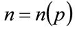
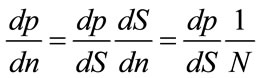
Let n be the number of consumers in the target population prepared to pay at least p, i.e. having a MAP of p, for the good, so that:
 (1)
(1)
Assuming a constant variable cost per item,  , and letting the fixed costs be
 , the retailer’s profit will be:
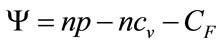 (2)
(2)
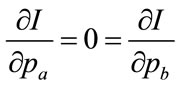
Since n is a function of MAP, the maximizing condition,  , may be written formally as:
 (3)
(3)
Provided the rate of change,  , in the number, n, of people in the target population prepared to pay at least p for the good is non-zero, the maximizing condition of Equation (3) implies
 provided
 (4)
(4)
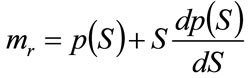
Thus differentiating Equation (2) gives the profitmaximization condition as
 (5)
(5)
Here  is the revenue at price, p, while
  represents the costs. Since differential operator,
  , denotes marginal with respect to the number of sales, Equation (5) corresponds to the standard economic finding that the maximum profit occurs when marginal revenue,
  , equals marginal costs:
  . Thus the profit maximizing condition has the form:
 (6)
(6)
where the marginal revenue is given by
 (7)
(7)
The bracketed term, (n), emphasizes that the price, p, is related to the number, n, of consumers prepared to pay at least that amount.
The fraction of the target population of consumers prepared to pay at least p for the good is . Differentiating that expression with respect to n gives:
 (8)
(8)
Moreover,
 (9)
(9)
Substituting from Equation (9) into Equation (7) gives the marginal revenue as:
 (10)
(10)
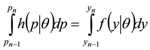
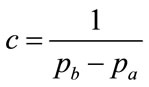
The price, p, is related to the number,  , willing to pay that price or more for the good by the probability distribution for MAP, p, or demand density,
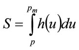
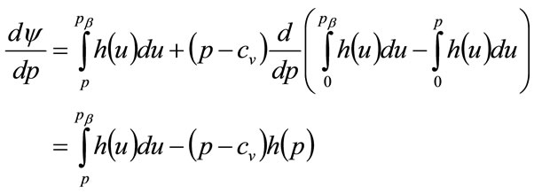
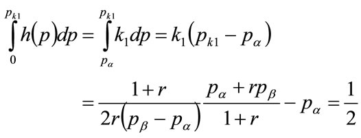
  , as illustrated in Figure 1. Meanwhile the fraction of consumers prepared to pay price p or more is given by:
 (11)
(11)
where  is the highest MAP for anyone in the target population, the maximum price anyone is prepared to pay.
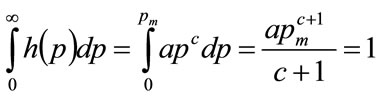
By the properties of a probability distribution,
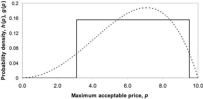
Figure 1. Examples of Double Power demand density, h(p), and Rectangular demand density, g(p).
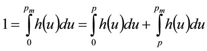 (12)
(12)
Substituting from Equation (12) into Equation (11), we achieve the relationship between price, p, and the fraction, S, prepared to pay at least that amount as:
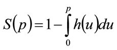 (13)
(13)
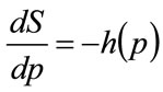
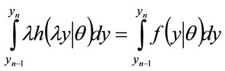
Differentiating Equation (13) with respect to p gives:
 (14)
(14)
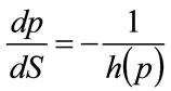
and so
 (15)
(15)
Substituting into Equation (10) gives the marginal revenue as:
 (16)
(16)
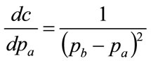
The conventional demand curve may be found by plotting on the graph of p vs. , the additional functions:
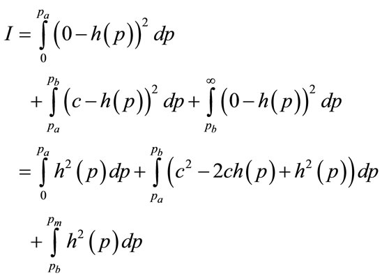
• the marginal revenue,  (found from Equation (16)), versus S
• the marginal cost,  , versus S.
See Figure 2, which may be compared with, for example, Figure 13.3 of [1].
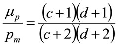
2.2. Equivalence between the Two Curves for a Double Power Demand Density
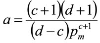
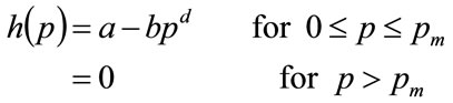
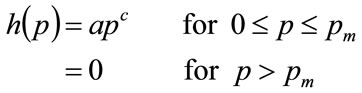
The Double Power demand density, which will be discussed more fully in Section 4, is defined on non-negative values of MAP, p, by
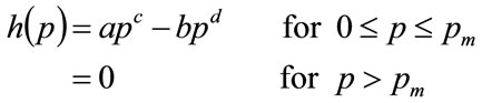 (17)
(17)
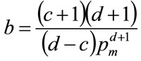
Where a, b, c and d are non-negative constants, and  is the highest MAP for anyone in the population. It will be shown in Section 4 that, if the mode is strictly interior to the interval,
  , then the coefficients, a and b, are given in terms of the powers, c and d and the highest MAP,
  , by:
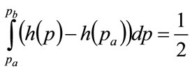
, by:
 (18)
(18)
 (19)
(19)
Hence, within the range of interest,  , the fraction of the population prepared to pay at least price, p, is
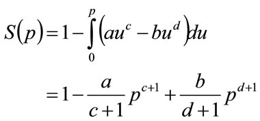 (20)
(20)
The marginal revenue at this value of S is given using Equation (16)
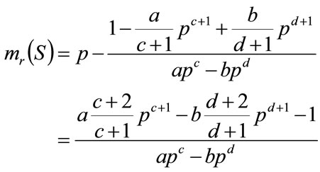 (21)
(21)
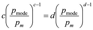
The condition of optimality using the demand curve approach is , which implies
 (22)
(22)
Substituting for a and b gives:
 (23)
(23)
Multiplying throughout by , and denoting the optimal price by p* gives:
 (24)
(24)
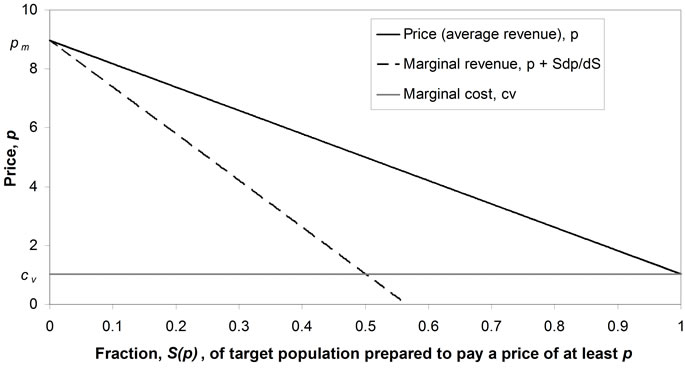
Figure 2. Conventional demand curve.
Equation (24) matches Equation (67) derived from the direct optimization procedure explained in Section 4.
2.3. Equivalence between the Two Curves for a Rectangular Demand Density
The demand density,  , for a general Rectangular distribution for MAP, p, is given by:
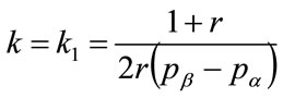
 (25)
(25)
Using the probability density,  , in place of
  in Equation (13) gives
 (26)
(26)
The function may be rearranged to give p explicitly in terms of S:
 (27)
(27)
Meanwhile, from Equation (16)
 (28)
(28)
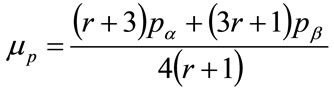
Substituting from Equation (27) into (28) gives the result that is the basis of the straight-line graph often used in economic text books:
 (29)
(29)
Thus when a Rectangular distribution is used to represent the MAP, then the demand curve is a downward sloping straight line (Equation (27)), while the marginal revenue curve is also a downward sloping straight line, with twice the gradient (Equation (29)).
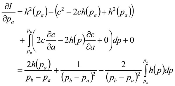
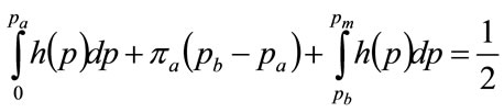
Since the optimal price occurs when , using Equation (28) and then Equation (26) to eliminate S, we have:
 (30)
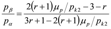
(30)
So that the optimal price is
 (31)
(31)
Assuming that the retailer will expect  and the lower limit of his mental model for the MAP to coincide, so that
  [4], then the optimal price is simply
 (32)
(32)
The same as the mean of the Rectangular demand density for MAP. The result coincides with Equation (10) of [4].
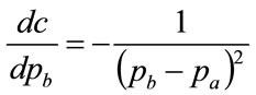
3. Relating the Demand Density to UK Post-Tax Household Income Percentiles
This Section addresses the problem of relating demand densities to the willingness to pay as measured by UK post-tax household income. The income percentile will be shown to be equivalent to the cumulative probability of a household chosen at random having an income less than the specified amount. The relationship between this cumulative probability and an associated cumulative probability for MAP will be established. Mathematical reasoning then produces the necessary relationship between demand density and probability density for the income of a cohort at a given percentile. Data on income may be available only cumulative form, in which case the demand densities need to be found by numerical differentiation, so that they will emerge as staircase functions. Since the method of matching the Rectangular demand density to the underlying demand density presented in Section 5 relies on the latter being continuous, it is necessary to fit a polynomial to portions of the staircase function, with a quadratic giving adequate accuracy.
3.1. Household Post-Tax Income and Income Cohorts
The data on income are often available only in cumulative form. Thus Figure 3 shows the cumulative probability for the post-tax income, x, of a UK couple with no children [5]. The data are presented in the format of the “Modified OECD” equivalence scale, in which an adult couple with no dependent children is taken as the benchmark with an equivalence scale of 1.0. This “equivalised income” is intended to allow comparability between all individuals within the nation.
Let x be a household income level, and let  be the cumulative probability of a household, chosen at random, having an income, X, up to x (£/y):
 .
.
Associated with this income level, x, will be a figure,
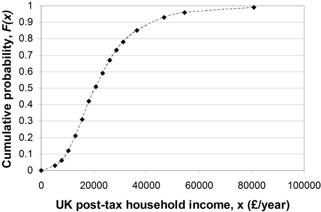
Figure 3. Cumulative probability versus UK post-tax household income 2009.
 , for the percentage of households having that income, x, or lower:
 (33)
(33)
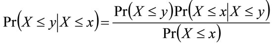
Let that income be called the  -percentile income and let the
  -percentile cohort be the collection of people whose household income is less than or equal to this income, x. Now choose an income level, y, less than or equal to x. The conditional probability that a household chosen at random has an income level, X, satisfying
  given that the household is known to be a member of the
  -percentile cohort follows from the basic tenets of probability theory:
 (34)
(34)
But since , it follows that:
 . Hence, using the notation:
 , Equation (34) becomes:
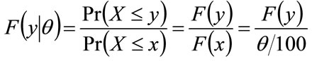 (35)
(35)
Thus, for any two cohorts defined by income levels,  and
and , with associated cumulative percentages,
  and
and ,
,
 (36)
(36)
Hence by setting , any conditional distribution,
  , may be calculated from the unconditional distribution,
  , using Equation (36).
3.2. Relating MAP to Income Cohorts
Assume that the maximum amount that people will be prepared to pay for each good is proportional to their income. Thus the maximum any person is prepared to pay, his MAP, p, measured in £, will be proportional to his ability to pay, y , as measured by his post-tax household income, in £/year: , where
  is a constant of proportionality. The highest MAP, the maximum that anyone in the
  -percentile cohort will prepared to pay,
  , will be dependent on the highest income in that cohort, viz.
 , where
  is the maximum income earned by anyone in the cohort. Meanwhile, cohort members in any income bracket
  will have MAPs in the range
 . Thus the number of people with a MAP between
  and
and  will be the same as the number with incomes between
  and
and . Therefore the following relation will hold, between the cumulative probability density for MAP,
  , and the cumulative probability of income, for the
  -percentile cohort:
 for all
 (37)
(37)
Because both incomes and MAP may both fall to zero but not go below this value, i.e. , then:
 for all
 (38)
(38)
It follows that Equation (37) may be applied successively, starting from , to give
 (39)
(39)
The cumulative probability densities,  , may now be used to estimate the probability density for MAP,
 . (The paper will use the convention that the highest MAP in the
  th percentile cohort will be set at 10 units of currency:
  for each value of
 . Hence
  will be defined on
  for all
 .)
.)
We may develop also the relationship between the probability density for MAP,  , and the probability density for the income of the
  -percentile cohort, given by
 . Equation (38) implies:
 (40)
(40)
Since  and hence
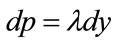 , we may change the variable of integration of the left hand side from p to y:
 (41)
(41)
Equating integrands shows that the probability density for MAP for people in the θ-percentile for income is related linearly to the probability density for income in that percentile:
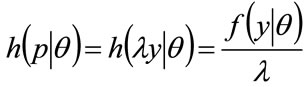 for
for (42)
(42)
3.3. Price Takers
To develop the MAP model further, assume that the price of commodities that are needed and obtained by all will be determined by the attitudes and decisions of those who have household incomes up to a certain percentile, the  th percentile. Those with incomes above the
  th percentile will then be price-takers for these goods. Clearly the valuation of some scarcer, desirable goods will require
  to be set high, very high for luxury goods such as high-performance sports cars and large residences in central London; the latter, particularly, are generally accepted as being the preserve of the super-rich.
The percentage,  , of people determining the price of each commodity may vary according to commodity, and moreover, that percentage may not be known with any precision. To cope with this situation, results may be derived for a range of possible percentages,
  , from 51% to 99%, for example. See Table 1.
3.4. Fitting a Staircase Probability Density to the Probability Density,  , for MAP for People with Income Below the θth Percentile
In the case where the data on income is available only in cumulative form, the demand density,  , needs to be found by numerical differentiation, and hence will emerge as a staircase function:
 (43)
(43)
By the properties of a probability density:
 (44)
(44)
So that combining Equation (43) with Equation (44) gives:
 (45)
(45)
Hence the coefficient,  , will be given by:
 for
for (46)
(46)
Applying the procedure to the data points marked in
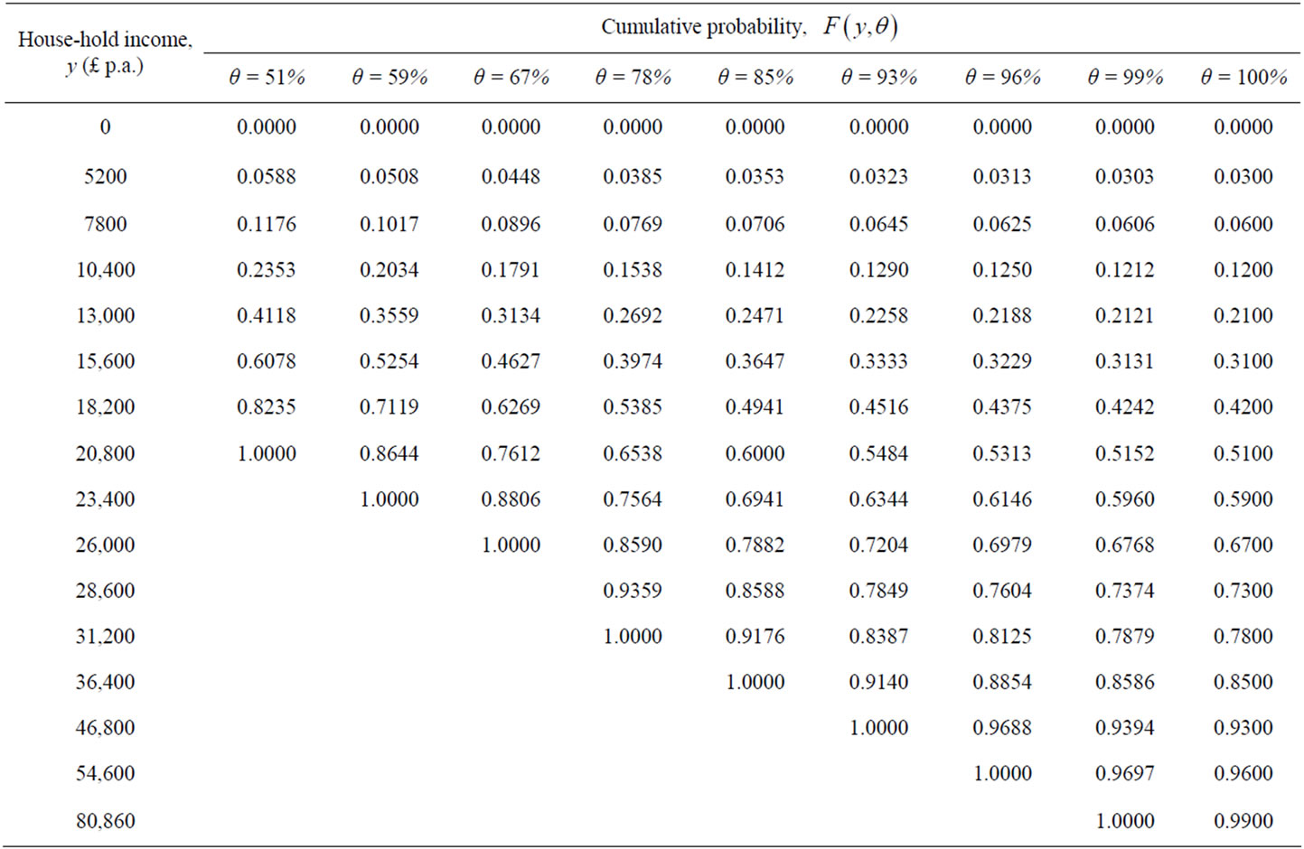
Table 1. UK post-tax household income 2009: Cumulative probability,  , up to the
  th percentile income (equivalised, based on a couple with no children).
Figure 3, produces the staircase probability density for MAP shown in Figure 4. It is clear from this figure that the probability density,  , resulting from this procedure is strictly unimodal.
The correctness of the procedure may be checked by integrating  from an initial condition of
 , utilizing the coefficients,
  , that have been found from Equation (46) and then employing Equation (44):
 (47)
(47)
Figure 4 shows two piecewise continuous probability densities that have been matched over the central section of the distribution. They have been chosen to be quadratics to allow ease of inversion, a convenient property used in the least-squares fitting of a Rectangular distribution. The process of fitting the quadratics will be discussed in the next section.
3.5. Smoothing Sections of the Staircase Probability Density Using 2nd Order Polynomials
The method of matching the Rectangular demand density to the underlying demand density (explained in Section 5 to follow) relies on the latter being continuous. Hence it
Figure 4. Staircase probability density for UK post-tax household income 2009. Quadratics matched to the portions of the curve above and below the mode.
is necessary to fit a polynomial to portions of the staircase function, with a quadratic giving adequate accuracy. Let the 2nd order polynomial approximation to the staircase probability density over the interval  take the form:
 (48)
(48)
where ,
,  ,
,  and
and . The optimal values of
  and
and  are taken to minimize the integral squared error:
 (49)
(49)
Then let the 2nd order polynomial approximation to the staircase probability density over the interval  take the form:
 (50)
(50)
where ,
,  ,
,  and
and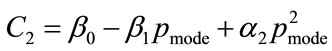 . The optimal values of
  and
and  are taken to minimize the integral squared error:
 (51)
(51)
The quadratics are, of course, convenient to invert. Rearranging Equation (51) gives:
 (52)
(52)
For the data shown in Figure 4, the positive root of the discriminant is needed, so that the general solution for the MAP, p, between  and
and  is:
is:
 (53)
(53)
Similarly, the general solution is for the MAP, p, between  and
and  is:
is:

 (54)
(54)
since the negative root of the discriminant is needed in this case.
4. The Properties of the Double Power Demand Density
This Section will derive the properties of the Double Power demand density for the three exhaustive and exclusive cases, namely 1) when the mode is strictly interior to the interval between zero, 2) when the mode is located on the lower boundary of the interval, viz. 0, and 3) when the mode is located on the upper boundary, viz. . The properties sought are the central measures characterizing any probability distribution, namely the mode, the median and the mean, and then the optimal price, which becomes a property of a demand density. Furthermore, the parameters,
  and
and , that define a Rectangular demand density matched to the underlying demand density become additional characteristics of that underlying probability density. These lead to a Rectangular optimal price that is simply the arithmetic average,
  , which becomes a further characteristic of the underlying demand density.
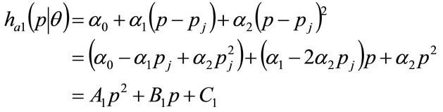
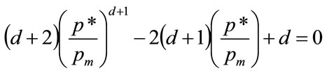
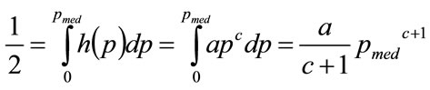
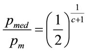
4.1. When the Mode Is Strictly Interior
For the general Double Power demand density defined by Equation (17), a strictly interior mode will occur when b > 0 and c > 0. Moreover, continuity implies that . Meanwhile it is a property of any probability distribution that its integral over all possible values will be unity. Hence:
 (55)
(55)
The solution of Equation (55) under the condition of continuity gives a and b in terms of the powers, c and d as:
 (56)
(56)
 (57)
(57)
The mode,  , occurs at the maximum value of
 , which will occur when
 (58)
(58)
Substituting from Equations (56) and (57) gives
 (59)
(59)
so that, on cancelling the term,  , we are left with:
 (60)
(60)
so that the normalised mode,  , emerges as:
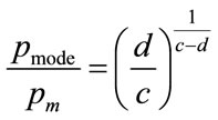 (61)
(61)
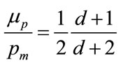
The mean is given by:
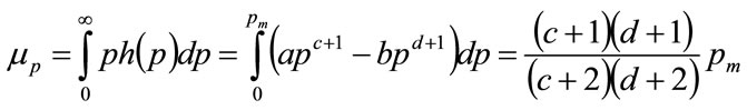 (62)
(62)
in which Equations (56) and (57) have been used to eliminate a and b. Thus the normalised mean,  , is given by:
 (63)
(63)
The median occurs when:
 (64)
(64)
so that, after substituting for a and b, the normalised median,  , is given by:
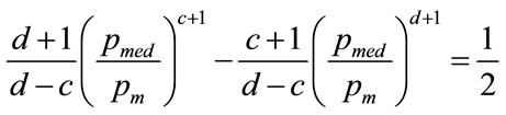 (65)
(65)
which Equation will normally require an iterative, numerical solution.
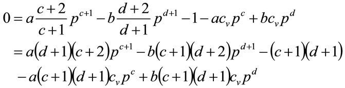
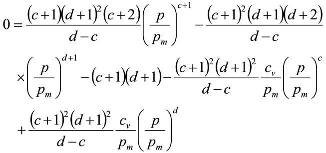
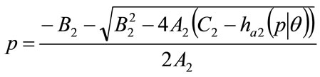
The optimal price,  , will be the solution to Equation (6) of [4]:
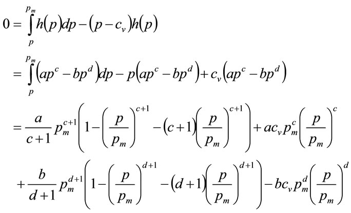 (66)
(66)
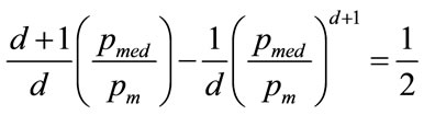
Substituting for a and b from Equations (56) and (57) and re-arranging gives the equation for the normalised optimal price,  , as:
, as:
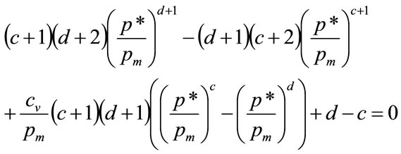 (67)
(67)
The condition for the least-squares fitting of a Rectangular demand density with base coordinates, ( ) and (
 ), is derived in Section 5 as Equation (100). This leads, in the case when the Double Power is the underlying demand density, to:
 (68)
(68)
Eliminating a and b and re-arranging gives the final expression
 (69)
(69)
Noting that  is the function of
  given in Equation (119) of Section 5.3, it is now possible to solve Equation (69) by iterating on
 , the normalised value of the lowest MAP in the Rectangular distribution.
4.2. When the Mode Occurs at p = 0
When c = 0, Equation (17) becomes
 (70)
(70)
where, from Equations (56) and (57):
 (71)
(71)
 (72)
(72)
The normalised mean,  , follows from putting
  into Equation (63), to give:
 (73)
(73)
The normalised median,  , is found by putting
  into Equation (65), to give:
 (74)
(74)
The condition for the least-squares fitting of a Rectangular probability density is given by Equation (102) from Section 5, which yields, in the case where ,
,
 (75)
(75)
Thus
 (76)
(76)
Combining Equations (72) and (76) provides an explicit solution for , the normalised value of the highest MAP in the Rectangular distribution.:
 (77)
(77)
Clearly  as
as  and
and  as
as , which will result in the mean value of the Rectangular distribution becoming 0.25 and 0.5 respectively.
The optimal value resulting from the Double Power probability distribution with c = 0 may be found from substituting c = 0, and also  into Equation (69):
 (78)
(78)
Clearly 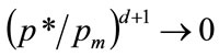 as
as 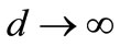 for the condition that the optimal price is strictly less than the maximum feasible price,
  , and this means, from Equation (78), that
  as
as . Limiting behavior can also be demonstrated by numerical solution as
 , when
 . Numerical calculation shows that
  rises from 0.2847 to 0.4995 as d increases from 0.001 to 1000.
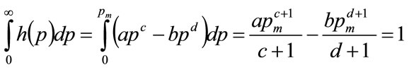
4.3. When the Mode Occurs at p = pm
When b = 0, the Double Power probability density of Equation (17) reduces to:
 (79)
(79)
The requirement for a probability distribution means that
 (80)
(80)
So that a is defined as soon as c and  are defined:
 (81)
(81)
The mode for this distribution will be . The mean value will be:
 (82)
(82)
where the last step follows the substitution for a from Equation (81). Hence the normalised mean,  , is given by:
 (83)
(83)
The median,  , follows from:
 (84)
(84)
Substituting for a and re-arranging gives the normalised median,  , as:
, as:
 (85)
(85)
From Equation (6) of [4] the optimum price is:
 (86)
(86)
Substituting for a from Equation (81) and re-arranging gives the normalised optimal price,  , as:
, as:
 (87)
(87)
The condition for the least-squares fitting of a Rectangular probability density is given by Equation (100) of Section 5. With the additional condition that , this yields
 (88)
(88)
Substituting for a from Equation (81) gives:
 (89)
(89)
Which gives the final expression for , the normalised lowest price in the Rectangular demand density as:
 (90)
(90)
For which a solution may be found by iteration.
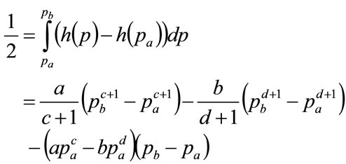
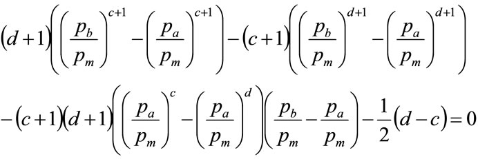
5. Optimal Matching of a Rectangular Demand Density to a General Unimodal Distribution
This section derives a method for matching a Rectangular demand density to a general unimodal demand distribution, based on minimizing the squared error between the two curves. The first subsection uses calculus, while the second shows the results in geometrical terms. Both the analytical first part and the geometrical second part are needed in order to devise a robust numerical method for the fitting procedure, as described in Section 5.3.
5.1. Optimal Matching Procedure
Let the general unimodal demand density be , defined on
 , where
  is the maximum possible price. The integral of the squared error between the general distribution,
  , and the Rectangular demand density with vertical legs at
  and
and , will be:
 (91)
(91)
where:
 (92)
(92)
Hence
 (93)
(93)
And
 (94)
(94)
The integral of Equation (91) will be minimized when
 (95)
(95)
Now the general integral:
 (96)
(96)
May be differentiated to give the following partial differentials:
 (97)
(97)
 (98)
(98)
Hence
 (99)
(99)
Noting Equation (95), we may write the first maximizing condition as:
 (100)
(100)
Moreover
 (101)
(101)
Applying condition (95) gives the second maximizing condition as
 (102)
(102)
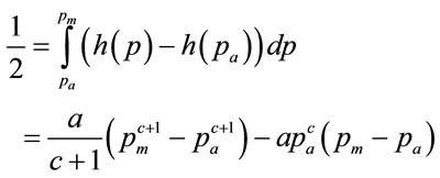
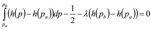
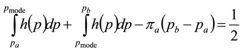
Comparing the integrands in Equations (100) and (102), it is clear that, at the minimum integral squared error,
 (103)
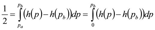
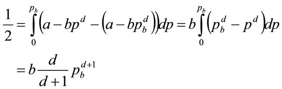
(103)
Since  as a consequence of h(p) being a probability density, it follows that the horizontal, straight line connecting
  with
with  will cut the locus of
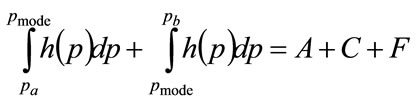
  so as to divide the area under the curve into two, with equal areas above and below the straight line. See Figure 5 and Section 5.2 below.
In the general case, Equation (103) and either Equation
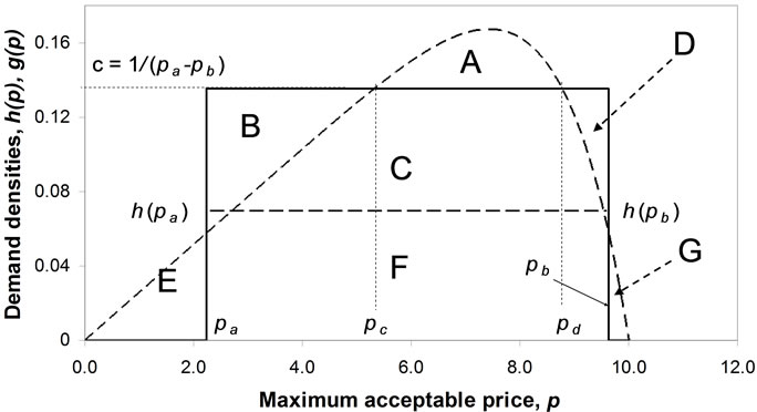
Figure 5. Fitting a Rectangular demand density, g(p), to a general demand density, h(p), with an interior mode.
(100) or Equation (102) need to be solved simultaneously for  and
and . One numerical procedure consists of iterating on the two values,
 ,
, , so as to satisfy
 (104)
(104)
where  may take any value;
  may be recognized as a Lagrange multiplier.
When the best fit occurs with either  or else
 , one of the minimizing variables,
  , will drop out of the optimization process, and the horizontal line is lost. In the case where
  is fixed at the top end of the interval, viz.
 , then only Equation (100) needs to be solved for
 . If
. If  is fixed at the lower end of the interval:
 , then only Equation (102) must be solved for
 .
.
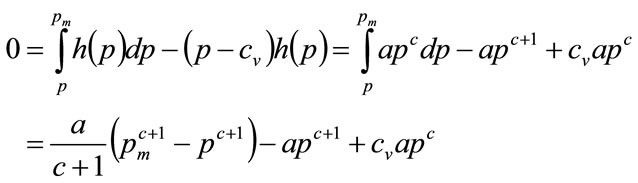
5.2. Geometrical Considerations
As will be seen, geometrical considerations allow a more robust numerical algorithm to be developed. Referring to Figure 5, since the area under the probability distribution,  , defined on (
 ), must equal unity, it follows that
 (105)
(105)
The area under the Rectangular probability distribution,  , defined on (
 ), must equal unity also. Hence:
 (106)
(106)
Eliminating the area,  , gives:
 (107)
(107)
which means that the integrated error will be zero. Equation (102) implies that
 (108)
(108)
Thus combining Equation (108) with Equation (105):
 (109)
(109)
Positive areas, E or G or both, will imply .
.
It has been shown in Section 5.1 that the lower line bounding the area, C, must be horizontal ( , see Equation (103)). Hence
 (110)
(110)
A positive area, E, implies
 for some
 (111)
(111)
While a positive area, G, implies
 for some
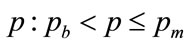 (112)
(112)
Either or both of conditions (111) or (112) will entail
 (113)
(113)
So that
 (114)
(114)
Equation (114) adds an additional constraint to the optimization Equation (104) for the important case where the probability density has positive values throughout the range,  , that is to say when
 for all
 (115)
(115)
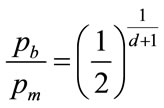
The limiting case, where inequality (114) becomes an equality, viz.:
 (116)
(116)
Occurs when the area, F, and the sum of areas,  , each becomes 0.5:
 (117)
(117)
Equation (117) applies when , when the probability distribution being matched would need to have the same base as the Rectangular distribution. It might, indeed, be a Rectangular distribution, implying a perfect match, but, conceivably, it could be some other distribution, albeit a somewhat unusual one, such as a rectangle of height
  topped by a triangle of height
 .
.
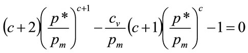
5.3. Numerical Method for Fitting a Rectangular Demand Density to a General Unimodal Distribution
Successively better estimates may be made of the two prices,  and
and , so as to satisfy Equation (104) more exactly, subject to the constraint of Equation (115), but the process is not always well conditioned. An alternative is given in this section.
Knowledge of the unimodal probability density function,  , for MAP, p, allows us to invert the function (e.g. via a numerical table):
 (118)
(118)
Using Equation (103), we may write:
 (119)
(119)
From Equation (109):
 (120)
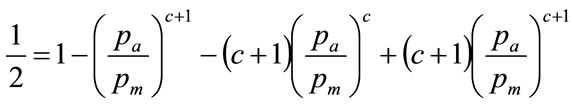
(120)
Equations (103), (119) and (120) now form an implicit equation set in the single unknown, .
.
Alternatively, it follows from Figure 5 that
 (121)
(121)
Equation (121) may be reduced using Equations (103) and (110) to:
 (122)
(122)
which is an alternative expression to Equation (120).
Making use of the intermediate transformation
 (123)
(123)
we may choose to iterate on  rather than on
  when the mode is close to zero, and
 .
.
6. The Properties of the Kinked Demand Curve
The kinked demand curve [6], [7], may be seen as an asymmetric combination of the assumptions made by Bertrand [8] and Cournot [9] about the behavior of an oligopoly. The construct has caused controversy amongst those economists who considered the rapid adjustment of prices a fundamental economic tenet [10]. The present authors make no case for or against the kinked demand curve, but include it as a method that has been used to represent demand under oligopoly.
6.1. The Equivalence of the Kinked Demand Curve and the Kinked Demand Density
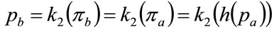
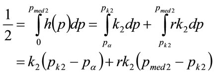
Referring to Figure 6 for the notation, assume the Kinked demand density,  , is given by
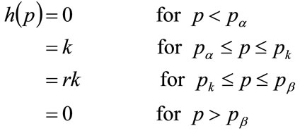 (124)
(124)
Applying Equation (13) gives
Figure 6. Kinked demand density defining k, r, pα , pk and pβ.
 (125)
(125)
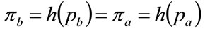
Moreover, 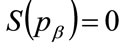 , which implies from the second part of Equation (125) that the following relationships hold:
 (126)
(126)
And
 (127)
(127)
Hence Equation (125) may be rearranged to give p explicitly in terms of S:
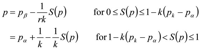 (128)
(128)
Equation (128) is the equation of the kinked demand curve, as shown in Figure 7, which includes the marginal revenue calculated from Equation (16). It may be noted that Figure 7 gives the demand curve for the target population, defined by those whose MAP lies in the range: .
.
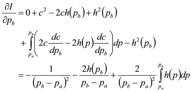
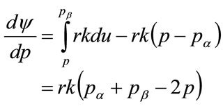
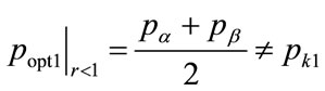
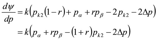
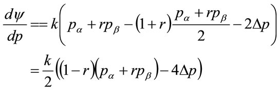
6.2. The Optimal Price
For a constant population, with each buyer purchasing one item, the optimal price implies maximization of the profit per person,  , for which a necessary, but not sufficient, condition is that
 . Using Equation (5) of [4], but now with
  replacing
  as the
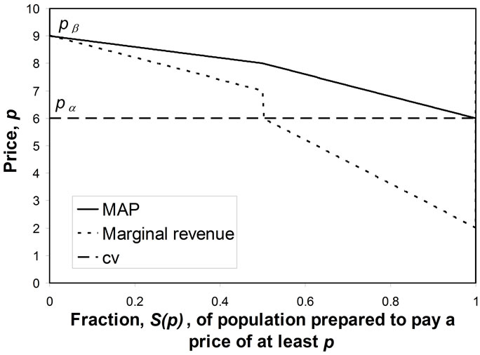
Figure 7. Demand curve when: r = 2, pα = 6, pβ = 9.
maximum price that will achieve a sale, gives
 (129)
(129)
The assumption is made that the rational retailer will expect  and the lower limit of his mental model for MAP to coincide:
 , as discussed in Section 4 of [4]. Equation (129) will be valid for prices, p, above and below the kink price,
 . For the case where
 , Equation (129) becomes, after putting
 :
:
 (130)
(130)
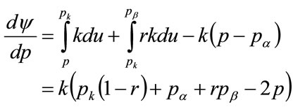
Applying the necessary requirement for optimality namely that , the optimal price will be
 (131)
(131)
Moreover, differentiating Equation (130) gives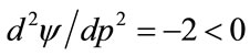 , confirming a maximal point. We may constrain the optimal price to be equal to the kink price, so that there is a incentive for stable trading at this price, in which case:
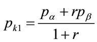 (132)
(132)
where the extra subscript “1” has been added because it is necessary to consider, in addition, how  changes beyond the kink point. For higher prices the following equation holds for the rate of change of profit per person with price:
 (133)
(133)
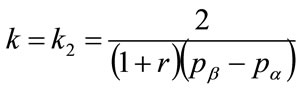
Setting  to zero, this implies an optimum at a different price, which is a second candidate for the kink price:
 (134)
(134)
For the first kink price,  , to give rise to stable trading, it needs to preserve its optimality over prices above the kink price:
 . This may be examined by substituting
  into the expression for the profit derivative when
 , Equation (133):
 (135)
(135)
Substituting for the first kink price,  , from Equation (132) gives, after re-arrangement:
 (136)
(136)
Since , it is clear that, when
 , the profit per person,
 , will fall if the retail price is set above
 :
:  at all positive values of
 . Thus it is clear that, provided that
 , entailing an upward step in probability density and hence a concave kinked demand curve, the profit will reach an overall maximum at a kink price of
 . This will enable stable trading at that value.
Such stability is will not occur at a kink price of  if
if , implying a convex kinked demand curve. The profit per person will now tend to rise,
  , as the price is moved just above
 . The overall optimal price will now be that which pertains in the region above the kink, and therefore given by Equation (134):
 (137)
(137)
To examine the validity of the second candidate for the kink price,  , we substitute
  and
and  into the expression for the profit derivative when
 , Equation (130):
 (138)
(138)
Substituting for  from Equation (134) gives:
 (139)
(139)
Hence, if the retail price is set below , viz.
 , then the profit per person is guaranteed to rise,
 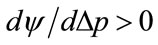 , if
, if  and the kinked demand curve is convex. For
 and
and , corresponding to a concave kinked demand curve,
  when
when 
 , indicating a local maximum. When
  a global maximum is indicated, as has been confirmed by numerical calculation.
Thus for a concave kinked demand curve, where , it is possible for the same values of
 ,
,  and r to have two different values for the kink price,
  and
and , given by Equations (132) and (134).
Consider the case of a convex kinked demand curve, viz. , when the kink price is set at
 . The price giving the overall maximum profit per person may be found by substituting for
  from Equation (134) into Equation (131):
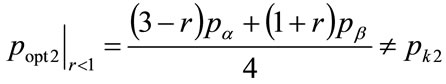 (140)
(140)
It may be seen from Equations (137) and (140) that when  and the kinked demand curve is convex, neither setting the kink price at
  nor setting it at
  will cause the kink price and the optimal price to coincide. Hence there will be no incentive for a retailer to continue trading at the kink price when the kinked demand curve is convex. This suggests that the construct of a convex kinked demand curve, as suggested as a variant by Sweezy [7] in his Figure 2, does not represent a situation of stable trading. Hence convex kinked demand curves will not be considered further in this paper.
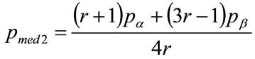
6.3. Central Measures of the Concave Kinked Demand Curve
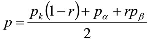
As a preliminary, substitute  into Equation (126) and use Equation (132) to give
 (141)
(141)
and  into Equation (126), now using Equation (134) to give
 (142)
(142)
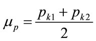
The mean value of the Kinked demand distribution may be calculated from:
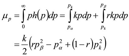 (143)
(143)
When  and
and , substituting into Equation (143) from Equations (132) and (141) gives, after re-arrangement:
 (144)
(144)
When 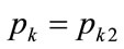 and
and , substituting into Equation (143) from Equations (132) and (141) gives
 (145)
(145)
which reduces to the same form as Equation (143): the same mean value pertains whether the kink price is  or
or . Moreover, it follows from Equations (132) and (134) that the mean price is the average of the two possible kink prices:
 (146)
(146)
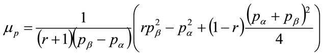
Now consider the integral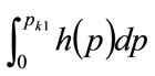 :
:
 (147)
(147)
Since the median,  , is defined by
 , it is clear that, when the kink price is set at
 , the median coincides with it:
 (148)
(148)
When the kink price is set at , the median,
  , will be defined by:
 (149)
(149)
Making the necessary substitutions from Equations (134) and (142) gives, after re-arrangement, the median price when the kink price is .
.
 (150)
(150)
The mode will occur between  or
or  and
and .
.
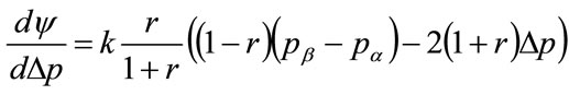
6.4. Contour Plot for Kinked Demand Curves
The ratio,  may be found by dividing Equation (143) by Equation (132)
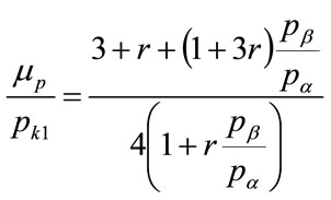 (151)
(151)
which may be recast into the form:
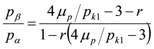 (152)
(152)
to enable a contour plot to be drawn with the price ratio,  , plotted against the post-kink slope multiplier, r, on the horizontal axis, with the ratio of the mean price to the optimal, kinked price,
  , as parameter. See Figure 8.
A similar set of curves are plotted in Figure 9 for , based on the analogous equation:
 (153)
(153)
It is clear from these two figures that the mean price and the optimal (kink) price are similar,  , for a
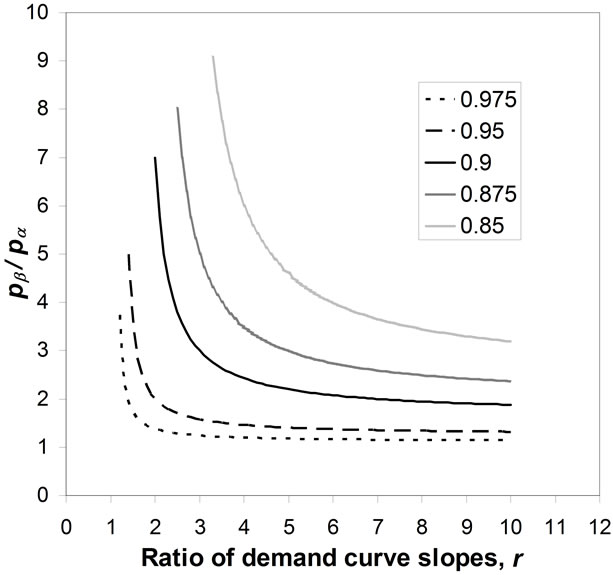
Figure 8. Kink price = pk1: contour plot with the ratio of mean price to the optimal price, μp/pk1, as parameter.
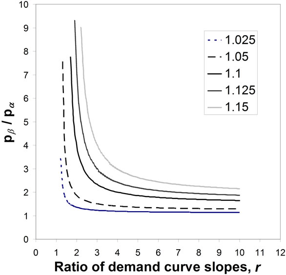
Figure 9. Kink price = pk2: contour plot with the ratio of mean price to the optimal price, μp/pk2, as parameter.
wide range of kinked-curve parameters.
By modifying the approach used in Section 5, it can be shown that the best-fit Rectangular demand density shares the same base as the Kinked demand density, so that  and
and .
.
7. Conclusions
The demand density curve has been shown to be equivalent to the demand curve conventionally used by economists. It has been shown that the demand density curve can offer a sharper picture of consumer demand than the conventional demand curve. The straight-line demand curve often used by economists as an exemplar has been shown to be equivalent to a Rectangular demand density, the simplest model of demand that may be useful to a retailer.
Derivations have been made of the properties of four demand densities of potential importance to retail price investigation, starting with the Household Income demand density, based on the assumption that a person’s MAP for a retail item will be proportional to his post-tax household income. The notion has been introduced that prices may be set by the retailer’s interaction with consumers earning incomes up a certain percentile, with those with incomes above that level being price takers. Mathematics has been presented relating the demand density to the probability density for income up to a given percentile. The process for translating cumulative probabilities for income into demand densities has also been explained, and a technique has been given for smoothing the results to facilitate later, optimal matching by a Rectangular demand density.
The Double Power demand density allows the mode to be located anywhere within a price interval, including at the boundaries, by suitable choice of its four coefficients. Analytical derivations have been given for the mode, the mean, the median and the optimal price for the Double Power demand density in each of the three possible locations of the mode: at the lower boundary, strictly interior to the interval and at the upper boundary. In addition, the mean of the matched Rectangular demand density, equal to the optimal price, has been derived for each of the three instances.
The process of matching a Rectangular demand density to a general demand density has been explained, based on the minimization of the integral of the squared error between the Rectangular and the underlying demand density. The mathematical results have been interpreted geometrically and a numerical method has been devised that allows the numerical matching procedure to proceed rapidly and efficiently. The results have been applied to all the Household Income and Double Power demand densities considered.
The Kinked demand density has been derived from the kinked demand curve sometimes used to conceptualize the effects of oligopoly. The translation into the domain of demand density has facilitated the analysis of the convex kinked demand curve, showing that it will not lead to stable trading at the kink price because the optimal price will always lie elsewhere. By contrast, it has been shown that stable trading at the kink price can occur with a kinked demand curve that is concave. For the same overall upper and overall lower price defining the Kinked demand density and the same ratio of slopes, it is possible for either of two, similar kink prices to be optimal and thus promote stable trading at the kink price. The mean price and the median price for a Kinked demand density have been derived analytically. Moreover, it has been shown that the optimal price and the mean price will be similar for a wide range of parameters when the kinked demand curve is concave.
8. Acknowledgements
The authors are grateful to Sir John Kingman and Mr Roger Jones for their helpful and useful comments on earlier drafts.
REFERENCES
- R. G. Lipsey and K. A. Chrystal, “An Introduction to Positive Economics,” 8th Edition, Oxford University Press, Oxford, 1995.
- D. Begg, S. Fischer and R. Dornbusch, “Economics,” 3rd Edition, McGraw-Hill, London, 1991.
- G. F. Stanlake, “Introductory Economics,” 5th Edition, Longman, Harlow, 1989.
- P. Thomas and A. Chrystal, “Retail Price Optimization from Sparse Demand Data,” American Journal of Industrial and Business Management, 2013.
- Institute of Fiscal Studies (IFS), 2010. http://www.ifs.org.uk/wheredoyoufitin/
- R. L. Hall and C. J. Hitch, “Price Theory and Business Behaviour,” Oxford Economic Papers, No. 2, 1939, pp. 12-45.
- P. M. Sweezy, “Demand under Conditions of Oligopoly,” Journal of Political Economy, Vol. 47, No. 4, 1939, pp. 568-573. doi:10.1086/255420
- J. Bertrand, “Review of ‘Théorie Mathématique de la Richesse Sociale’ and ‘Recherches sur les Principes Mathématiques de la Richesse’,” Journal des Savants, 1883, pp. 499-508.
- A. A. Cournot, Recherches sur les Principes Mathématiques de la Richesse,” Chez L. Hachette, Paris, 1838. http://books.google.co.uk/books?id=K2VHAAAAYAAJ&printsec=frontcover&source=gbs_ge_summary_r&cad=0#v=onepage&q&
- G. Stigler, “Kinky Oligopoly Demand and Rigid Prices,” Journal of Political Economy, Vol. 55, No. 5, 1947, pp. 432-449. doi:10.1086/256581