Natural Resources
Vol.4 No.2(2013), Article ID:32897,9 pages DOI:10.4236/nr.2013.42023
Causalities between Price, Pond Area and Employment in Aquaculture Production
![]()
1Department of Economics, Faculty of Management and Economics, University of Malaysia Terengganu, Kuala Terengganu, Malaysia; 2Graduate School of Business, National University of Malaysia, Bandar Baru Bangi, Malaysia.
Email: nhm06@umt.edu.my, aqlina@umt.edu.my, nikhaz@ukm.my
Copyright © 2013 Nik Hashim Nik Mustapha et al. This is an open access article distributed under the Creative Commons Attribution License, which permits unrestricted use, distribution, and reproduction in any medium, provided the original work is properly cited.
Received January 29th, 2013; revised April 11th, 2013; accepted April 29th, 2013
Keywords: Aquaculture; Unit Root; Cointegration; Vector Error Correction Model; Granger’s Causality
ABSTRACT
The role of aquaculture industry is becoming more prominent in order to supplement marine capture in meeting the food need for the growing Malaysian population. In an attempt to minimize depletion of marine fisheries, only traditional vessels are allowed to fish along the coastal area while bigger vessels are relegated to deep-sea fishing. During the 9th Malaysian Plan (2006-2010) aquaculture has been recognized as the engine of growth in the national food sector’s development strategy. Future fisheries policy is expected to focus more on aquaculture production, marketing and technological improvement as an alternative to marine capture. This paper investigates the causalities between the selected freshwater fish prices, aquaculture area and production. The study aspires to establish whether or not market price is a key contributor to a rise in the aquaculture area and production. Aquaculture firms comprising the individual culturists are generally motivated by the economic potential of the industry which is reflected in excess of price over cost of production. Our hypothesis is that government policy and initiation rather than prices had give rise to greater participation of culturists and hence augmented the level of employment. However, production increase has a negative implication on environment degradation. Thus there is a conflicting view as regards to the employment opportunity generated by aquaculture undertakings and the need for sustainable development arising from this growing industry. Multivariate time series analysis was used in this investigation.
1. Introduction
The popularity of aquaculture practice in Malaysia comes with its commercialization during the last few decades. As such aquaculture is dominated by several fishery species associated with the market potential which is primarily reflected in high prices offered to the breeders. These fisheries are in fact experiencing shortage in supply. Species such as giant prawn (Macrobrachium rosenbergii) and tiger prawn (Penaeus monodon) are delicacies of hotels and restaurants due to the high demand while the supply is limited. Another underlying factor for their high demand is that special fishery species like the catfish (Clarias gariepinus) is believed among the majority of its medicinal healing capability. However, the success of culturing these aquatic resources either freshwater or brackish-water fisheries is always constrained by the economic factors such as high capital outlay to start the business and the expertise knowledge required in their breeding and maintenance. Availability of fingerlings, cost of feeding ingredients, suitability of land area in terms of location and lastly problems related to marketing and distributional system could be the salient factors that need to be considered in aquaculture practices.
In macro perspective aquaculture fishery is an essential component of the economy food security and sustainability. In 2009 the aquaculture statistics on area, production and the number of culturist were 4916.2 km2, 21,051 metric tons and 70361.5 persons respectively. The retail value accounted for about RM476, 549.45 for 2009 [1]. These statistics show continuous growth trends over the years indicating that the aquaculture industry is escalating perhaps due to the fact investors are attracted to the profitability of the prospective species. With an increase in demand for food owing to ever-growing population and heavy reliance of the present fishery policy on marine capture, the crucial function of aquaculture as supplementary to marine fisheries becomes obvious. By the end of the 9th Malaysia Plan 2010 Malaysia targeted to produce some 507,550 metric tons of aquaculture and aquatic products under the National Agricultural Policy [2]. Aquaculture is seen as an alternative that could reduce the pressure of over fishing on marine fisheries resource. The role of aquaculture in food economy is stipulated to become more important in future in view of depleting marine fisheries. In the light of this changing scenario which the government has agreed to adopt this as a new fisheries policy it deems necessary to investigate the extent to which interactions between pricing, area and employment are intertwined in order to provide economic rationale.
The objective of this study is to investigate the interdependencies of economic policy variables namely prices of freshwater fisheries, area invested with aquaculture ponds and the number of culturists. The general hypothesis is that although aquaculture provides the best alternative to marine capture its growth depends on the economic interplays of fish prices and aquaculture area. In big cities land competes for alternative investments pushing land price extremely high. Since the investment in aquaculture activity generally requires high initial capital, technical knowhow on fisheries rearing, difficulty of getting seedlings, high percentage of fish mortality due to river pollution, investing in aquaculture is almost impossible. Culturally majority of Malaysian favor marine fisheries it is therefore, hypothesized that the probability of a significant increase in aquaculture operators and thus employment is minimal. The results of this investigation are useful for decision makers in formulating strategic fisheries policies. If price is highly significant and correlated with employment and area cultured or otherwise, then strategic policy can be under-taken to further support such relationships.
2. Freshwater Catch and Production
Statistics provided by AQUASTAT [3] show that freshwater catch in 1990 was estimated at 12,995 metric tons about 10 percent of the total catch of 3,783,743 metric tons in Asia (excluding Middle-East). Freshwater catch for 2000 figures were 22,636 metric tons and 5,959,055 metric tons for Malaysia and Asia respectively. The catch difference is about 12 percent but there is an improvement of about 2 percent per annum over the period 1990-2000. The total share of aquaculture for Malaysia in terms of Asian aquaculture production in 1997 was relatively small which accounted for only 5 percent.
One of the more recent developments in aquaculture species of market potential is the red hybrid tilapia (Oreochromis sp.), a genetic improvement with attractive red coloration. In 2007 Malaysia produced 32,258 metric tons (80% red tilapia and 20% black tilapia) with the wholesale value of MYR170.6 million [4]. According to the same source fresh water red tilapia production constitutes about 46 percent of total aquaculture production and 12 percent of this total is from brackish water. In value term the production of tilapia is currently leading all other aquaculture species constituting 49.4 percent, followed by catfish 37 percent and carps 10 percent. The major drawbacks in aquaculture, in particular, the red hybrid tilapia production are soaring feeds cost, shortage of trained workers, diseases resistance fries and the supply of fingerlings has to be bought from commercial firms. The Institute of Tropical Aquaculture of the University Malaysia Terengganu (UMT) is doing research to produce diseases resistant seeds of tilapia.
The major drawback during the earlier part of freshwater development in this country originated from the domination of the marine capture over freshwater species and the consumers’ preference for the former. Over the last decade marine capture had experienced drastic changes due to depletion of the resource partly caused by the increased demand as population and income grew. On the supply side depletion of the resource is attributable to several factors, namely the continuous application of efficient fishing methods such as trawlers, the encroachment of efficient vessels from outsiders within the Malaysian 200 nautical miles Exclusive Economic Zone (EEZ), ineffectiveness policing of the fishing grounds owing to insufficient enforcement officers to guard the assigned EEZ. Aquaculture investment had been in Malaysia for a long period of time but had been tried on a relatively small scale because of the high risk and large capital needed for the industry. Hence, with existing requirement for additional supply of fish in addition to marine capture this industry started to flourish partly due to the aquaculture potential for sea food industry.
Experience shows that the success of aquaculture investment is likely to benefit the large scale operators more relative to small operators pertaining to the technical knowhow, culturing and breeding practices. In delivering their products contracts with the local hotels are made and for exporting fish products to destinations outside the country approval and procedures need to be adhered. The small operators with limited working capital, technical knowhow and access to the target market would be greatly at the disadvantage. Alternatively small operators could make this aquaculture undertaking a success through fishermen Association or Cooperatives. Otherwise the government policy that attempts to motivate culturists on an individual basis would be constrained by those farming practices, technicalities of making contracts and the delivery system requirements.
3. Materials and Methods
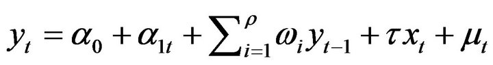
The theoretical discussion of the econometric multivariate model is discussed in Enders [5]. For a general presentation we begin with Pesaran and Pesaran [6] augmented vector autoregressive model of order ρ that is AVAR (ρ)
 (1)
(1)
where  is an n × 1 vector of endogenous (jointly determined) variables, a0 is a drift, t is a linear time trend,
  is an m × 1 vector of exogenous variables, and
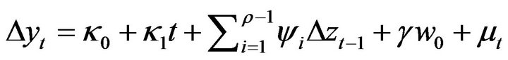
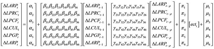
  is m × 1 vector of unobserved disturbance terms. The assumptions for the disturbance terms are the mean is zero, E(μt) = 0, not serially correlated E(μtμs) = 0, the variance matrix is time-invariant that is it does not vary with time. Since not all time series data representing these variables are stationary they have to be tested using Dickey-Fuller (DF) and augmented Dickey-Fuller (ADF) unit root statistics which is necessary in identifying their long-run cointegration [7]. Moreover, equation one contains a constant drift a0 and the linear time trend which has to be de-trended and to achieve the necessary condition for cointegration the non-stationary variables have to be differenced. The difference multivariate econometric equations exemplifying the general vector error correction model (VECM) [5] is shown in Equation (2) below
 (2)
(2)
where is an n × 1 vector of endogenous (jointly determined) I(1) variables.
 are ny × 1 vector of endogenous I(1) and nx × 1 exogenous I(1) variables respectively.
 is m × 1 vector of exogenous I(0) variables.
κ0 & κ1 are intercepts and deterministic linear trends.
 is n × 1 vector of unobserved disturbance terms.
T = 1, 2, …, T represents time periods.
Analysis of aquaculture development uses time series data 1976-2007 obtained from the Department of Fisheries annual statistics, the Ministry of Agriculture Malaysia. The objective of this investigation is to identify causalities between the freshwater fish prices namely that of giant prawn, catfish, river carps (Cyprinus carpio, Pangasius sp.) and goby (Gobiidae) with the total area (in cubic meter) of ponds devoted to rearing of these fresh0 water fisheries and the total number of culturists involved in the production activities. The multivariate equations for the model for the long run variables are presented in Equation (3).
An increase in the area of pond will attract more production of aquaculture into the market that acts to bring down the price of river carps and vice versa. Changes in the price of catfish will have both direct and indirect effect on the price of river carps depending on whether catfish compete or complement the river carps. While a rise in the number of culturists would increase aquaculture production that will ultimately reduce the price of river carps. Similar rationales can be used to explain the economic interrelationships for the rest of the equations in (3).
A direct impact on number of culturist a proxy for employment is anticipated from an increase in the area of pond. On the other hand, changes in either price of catfish or river carps will have a meaningful impact in terms of policy implication on the employment attraction to the aquaculture industry if the prices were found to be significantly associated with the number of culturists and vice versa. In the final analysis only the price of catfish (LPCF) was retained while the price of river carps (LPRC) was omitted from the endogenous system of equation for the long run cointegration analysis.
4. Results and Discussions
4.1. Stationary Tests
Table 1 shows results of unit root tests for the selection of variables that will be used in the multivariate equation model both with trend and without trend. At form level I(0) the number of culturists, the price of river carps and price of catfish were found to be stationary without trend. However, when the linear time trend is considered, with the exception of river carps price, all investigated variables were stationary at level I(0). The results at first difference revealed that all selected variables fulfilled the requirement for the stationary test since the estimated values were found to be greater than the Dickey-Fuller or the augmented Dickey-Fuller critical values as shown in Table 1 (see the Equation (3) below).
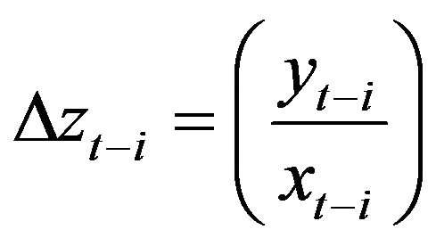
where, LARPt is annual area of freshwater pond in cubic meters at time t.
LPRCt is annual average price of river carps in MYR
 (3)
(3)
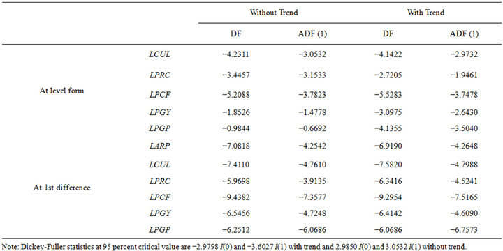
Table 1. Unit root tests for the related variables using dickey-fuller.
per kg at time t.
LPCFt is annual average price of catfish in MYR per kg at time t.
LCULt is annual total number of culturists in the industry at time t.
LPGYt is annual average price of goby in MYR per kg at time t, and LPGPt is annual average price of giant prawn in MYR per kg at time t.
All variables are measured in natural logarithmic values, ρ > 1 represents lag length greater than one, and ∆ is the difference notation. US$1 = MYR3.1.
 are intercepts of the multivariate equations,
 for i = j = 1, 2, ..., n
  represent the coefficients of endogenous and exogenous variables of the multivariate equations to be estimated in the model. The terms ecti refer to the error correction terms, whose coefficients measure speeds of adjustment and are derived from the long-run cointegrating relationships,
  represents the disturbance terms, and ρ is the lag lengths for the respective multivariable equations. Causalities tests between these endogenous variables in multivariate analyses using vector error correction model requires that each of these endogenous variables will be used as right hand side (RHS) equation as shown in Equation (3).
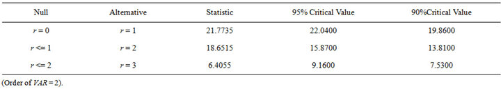
4.2. Number of Cointegrating Variables and Order of Lags
Tables 2(a) and (b) show the number of cointegrating variables, r, for the case of restricted intercepts and no trends in vector autoregressive (VAR) model. Both maximal eigenvalue and trace of the stochastic matrix suggest that at least the number of cointegrating variables, r = 2 for the order of lag, VAR = 2 at either 95% or 90% significant level respectively. Pesaran & Pesaran [5] caution that the figures reported by Microfit differ from those obtained by Johansen and Juselius [8] and also by Osterwald-Lenum [9]. However, results from the model selection Akaike Information Criterion (AIC), Schwarz Bayesian Criterion (SBC) and Hannan-Quinn Criterion (HQC) in Table 2(c) suggest the cointegrating variables of r = 3, r = 2 and r = 3 respectively. The cointegrating vectors based on the theoretical formulation of the endogenous variables that was originally intended for this investigation and those suggested using econometric criteria will be tested in order to get the most appropriate results. The lag order is limited to two after several trials were carried out for higher degree of lags had proven to yield no significant results. With higher degree of lags such as three and above the loss in the degree of freedom is somewhat serious given the limitation on the number of observations for this study.
5. Aquaculture Error Correction Model
Freshwater species which is widely raised by the majority of culturists is the catfish. Catfish species are relatively easy to breed and they are available in local markets. Furthermore, the species are believed by majority of Malaysians to have the specialty of healing capacity for bleeding. The price of catfish is relatively low compared to other freshwater delicacies like giant prawn. Hence, there is sufficient reason to believe that catfish prices
 (a)
(a)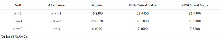 (b)
(b)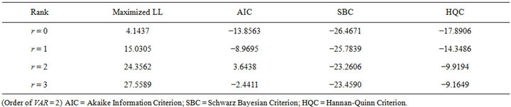 (c)
(c)
Table 2. (a) Cointegration with restricted intercepts and no trends in the VAR maximal eigenvalue of the stochastic matrix 1978-2007; (b) Cointegration with restricted intercepts and no trends in the VAR trace of the stochastic matrix, 1978-2007; (c) Cointegration with restricted intercepts and no trends in VAR using model selection criteria 1978 to 2007.
may have a significance influence in attracting culturists as well as the cultivated area for the long run cointegration analysis. These three policy variables are grouped as endogenous variables in the current study while the other prices of river carps, giant prawn and goby are included as the exogenous variables as they are being influenced by unobservable factors outside the currently available data.
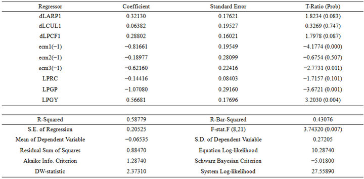
The log-linear error correction models (ECM) for the three endogenous variables namely the area per pond in hectares (dLARP), number of culturist (dLCUL) and average price of catfish (dLPCF) are shown in Tables 3 (a)-(c). These regression equations were first estimated using the ordinary least square (OLS) omitting their dynamic characteristics; that is, the differences and lags of the estimated endogenous variables are of order one I(1). The residuals have satisfied the necessary condition for the existence of long-run relationships.
The short-run characteristics of the ECM coefficients need to be substantiated from the difference equations of Table 3(a) thru Table 3(c). The Granger representation theorem (GRT) requires that the ECM coefficients are negatives and statistically significant.
As apparent ecm1(−1) =−0.81661 (Table 3(a)), ecm2(−1) = −1.0587 (Table 3(b)) and ecm3(−1) = −0.58028 (Table 3(c)) demonstrate that they are statistically significant at 99 percent probability level for the ecm1(−1) and ecm2(−1) respectively. The ecm3(−1) is also significant but at a probability level of 95 percent. Thus, the endogenous vectors used in current aquaculture study are cointegrated in the long-run. This is illustrated in Figures 1 thru 3 showing the impact of generalized impulse responses to one standard deviation shock on the cointegrated variables.
Further investigation of interest to the current study that utilizes the information given in Table 3(a) through Table 3(c) is to derive Granger’s causality test. According to Rosilawati Amiruddin et al. [10] the works of Granger [11], Hendry [12], Engle and Granger [6] and Johansen and Juselius [13] on the extension of cointegration technique had opened up new avenues for evidence of causalities in one and bi-directional which were once uncertain due to spurious regression results.
With cointegration between two or more variables and either one or bi-directional causalities could be carried out on appropriate model specification and this is done with the Wald test using Microfit. The section is discussed in next section under Granger’s causalities.
6. Granger’s Causality
Causality between variables in time series multivariate analysis was initially investigated by Granger [11,14]. In general it provides richer information than the single or univariate equation model because several endogenous and exogenous variables could be tested simultaneously. These causalities are obviously essential for identifying national strategies such as that on the current policy of promoting aquaculture to supplement the existing depleting marine fisheries. It looks reasonable to augment the present shortage of marine supply with aquaculture undertakings but it would be wise to further investigate and to ask; are the firms responsive to this strategy? They may not be responsive if the non-aquaculture investments outside the industry such as manufacturing, services and agricultural sector itself are more profitable and suitable
 (a)
(a)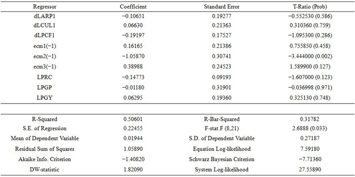 (b)
(b)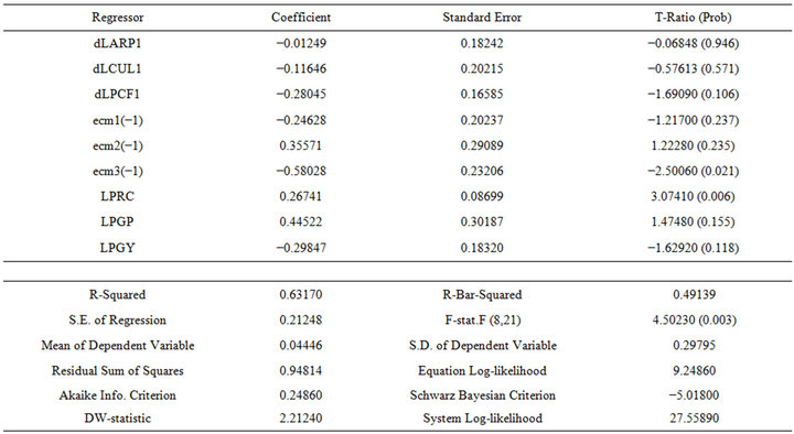 (c)
(c)
Table 3. (a) Log-linear ECM for dependent variable dLARP estimated by OLS based on cointegrating VAR (2), 1978-2007; (b) Log-linear ECM for dependent variable dLCUL estimated by OLS based on cointegrating VAR(2), 1978-2007; (c) Log-linear ECM for dependent variable dLPCF estimated by OLS based on co-integrating VAR(2), 1978 to 2007.
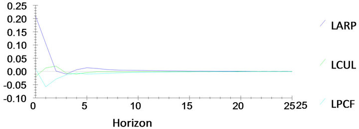
Figure 1. Generalized impulse response(s) to one S.E. shock for LARP.
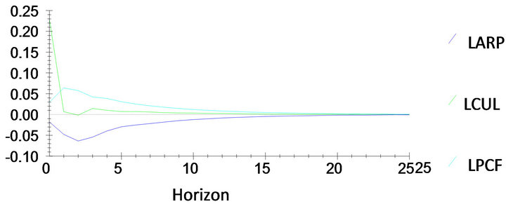
Figure 2. Generalized impulse response(s) to one S.E. shock for LCUL.
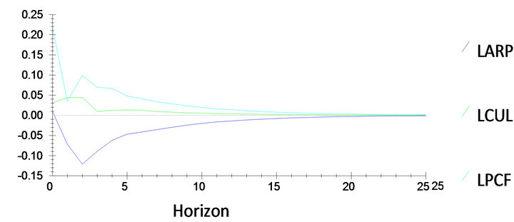
Figure 3. Generalized impulse response(s) to one S.E. shock for LPCF.
to the investors’ skills and interests.
Table 4 illustrates the existence of causality among the investigated economic variables in the Malaysian aquaculture industry. There should be either one, bi-directional or nonexistence of causality between these policy variables. The null hypothesis indicated that the size of aquaculture pond area (in ha.) had no causality whatsoever with the number of culturists in the industry and vice-versa. An increase in size of the aquaculture area had not contributed significantly to the course for raising employment. Alternatively, an increase in the number of culturists will not have the potential to increase the size of aquaculture area. However, changes in the one-period lag price of catfish (dLPCF), current prices of river carps (LPRC), giant prawn (LPGP) and current price of goby (LPGY) would draw a direct change in the size of aquaculture pond area. On the other hand, a change in price of catfish will have no effect on inducing one-period lag of size of aquaculture area (dLARP1).
With the exception of direct and current change in price of river carps that have some influence on changing the number of culturists, all other variables in the EVCM model apparently show no significant causality on culturists. Price of river carps may attract those anglers who fish for recreational purpose. Sometimes river carps can fetch a good price for local markets and restaurants and at other times organized competition in sea and river fishing are held. Private individuals also provide special fishing grounds for river carps and selected local freshwater fish species for anglers at reasonable fees.
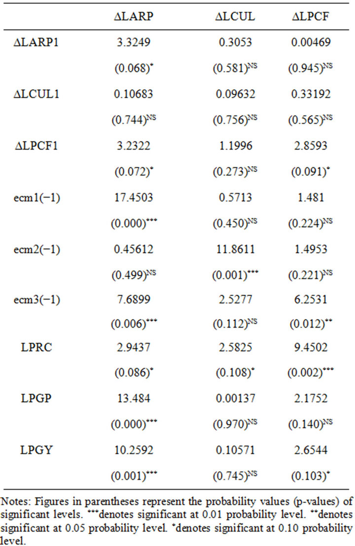
Table 4. Wald statistical tests for multivariate vector error correction model (VECM), 1978-2007.
The one-period lag catfish price (dLPCF1) has shown some degree of causality with its own current price
(dLPCF) at about 90 percent probability level. Similarly, the price of exogenous variable goby (LPGY) has exhibited some degree of causality on the current price of catfish. The degree of causality between the current price of river carps and the difference price of catfish are stipulated to be high at 99 percent probability level. In all of these cases the null hypotheses that support no causality between the prices mentioned above are rejected. It is true that the price of giant prawn has no association with the price of catfish. These species have their own market specialties.
In general, the finding revealed that price of catfish Granger causes the aquaculture area which is only onedirectional since the reverse influence of area on price is not significantly different from zero. Furthermore, the one-period lag aquaculture area Granger causes the current area and the one-period lag price of catfish Granger causes the current price of catfish. This trend is not observable in the case of number of culturists. The exogenous variables of the current prices of giant freshwater prawn, goby and river carps have greatly influenced the increase in size of the aquaculture area. The price of river carps and to a lesser extent the price of goby have a similar influence on the price of catfish. River carps and catfish are substitutes because their prices move in the same direction while goby and catfish are complementary products since their price movements are in the opposite direction.
7. Conclusions
The multivariate econometric vector error correction model was estimated using Microfit software to investigate the relationship between endogenous and exogenous variables namely the size of pond area, the number of culturists and the prices of the major fresh fish species. The findings revealed that price movements, specifically the price of catfish has caused changes in the size of the aquaculture pond area but the reverse is not true. This indicates that the direction of causality is one way. Furthermore, the potential of the variation in aquaculture area to draw larger investors as indicated by the number of culturists in the industry is most likely not going to happen. The causality between the determining variables is unfortunately insignificant, thus employment wise the promotion for aquaculture projects has not been able to place big hope in terms of employment generation. Possible explanations could be that aquaculture activities require a large amount of initial capital to start, high technical knowhow and it is a risky investment. This is without considering problems relating to marketing of fish harvests, getting supply of fries and the ever-increasing prices of land for fishponds compete with other economically potential investments. In the case of cage culture although it requires high initial outlays competition for water use is less profound; however, water quality needs to be assured from pollution.
The idea of utilizing freshwater and brackish water fisheries to supplement marine catch is nevertheless a worthy strategy that needs to be supported. However, special care for degradation of the environment due to aquaculture development and activities should be taken into consideration by the policy makers. Research and development should be conducted from time to time to find the best way to invest in aquaculture. It would be possible to allow individual households to start a small aquaculture projects to reduce costs and to be self-sufficient in food supply with fishery-based programs in addition to a several large privately owned aquaculture projects with government assistance.
8. Acknowledgements
The authors would like to express their grateful thanks to the Ministry of Higher Education for providing the financial support under the fundamental research grant scheme (FRGS) vote number 59189 for the duration of April 2009-March 2012. They also wish to thanks the unanimous reviewers of this article for their suggestions and recommendations.
REFERENCES
- Department of Fisheries Malaysia, “Annual Fisheries Statistics (1987-2007),” 2010. http://www.dof.gov.my/59
- Government of Malaysia, “Rancangan Malaysia Kesembilan 2006-2010,” Unit Perancang Ekonomi Malaysia, 2010.
- EarthTrends AQUASTAT, “Information System on Water and Agriculture Country Profiles,” 2003. http://www.fao.org/waicent/faoinfo/agricult/agl/aglw/aquastat/countries/index.stm
- P. J. Pradeep, T. C. Srijaya, H. Anuar, S. Faizah and C. Anil, “The Aquatic Chicken Tilapia and its Future Prospects in Malaysia,” Institute of Tropical Aquaculture, University Malaysia Terengganu, Terengganu. Prospect, Malaysian Premier Higher Education Magazine Times Guides Sdn Bhd, Pelangi Damansara, 2010, pp. 52-56.
- W. Enders, “Applied Econometrics Time Series. New Jersey,” John Wiley & Sons Inc., Hoboken, 2003.
- M. H. Pesaran and B. Pesaran, “Working with Microfit 4.0 Interactive Econometric Analysis,” Oxford University Press, Oxford, 1997.
- R. F. Engle and W. J. Granger, “Cointegration and Error Correction: Representation, Estimation and Testing,” Econometrica, Vol. 55, No. 2, 1987, pp. 251-276. doi:10.2307/1913236
- S. Johansen and K. Juselius, “Testing Structural Hypotheses in a Multivariate Cointegration Analysis of the PPP and UIP for UK,” Journal of Econometrica, Vol. 53, No. 1-3, 1992, pp. 211-244. doi:10.1016/0304-4076(92)90086-7
- Osterwald-Lenum, “A Note with Quantiles of the Asymptotic Distribution of the Maximum Likelihood Cointegration Rank Test Statistics,” Oxford Bulletin of Economics and Statistics, Vol. 54, No. 3, 1992, pp. 461-472. doi:10.1111/j.1468-0084.1992.tb00013.x
- A. Rosilawati, A. H. Shaari, and I. Ismail, “Test on Dynamic Relationship between Financial Development and Growth in Malaysia,” Gadjah Mada International Journal of Business, Vol. 9, No. 1, 2007, pp. 1-17.
- C. W. Granger, “Developments in the Study of Cointegrated Variables,” Oxford Bulletin of Economics and Statistics, Vol. 48, No. 3, 1986, pp. 213-227. doi:10.1111/j.1468-0084.1986.mp48003002.x
- D. F. Hendry, “Econometric Modeling with Cointegrated variables: An Overview,” Oxford Bulletin of Economics and Statistics, Vol. 48, No. 3, 1986, pp. 201-212. doi:10.1111/j.1468-0084.1986.mp48003001.x
- S. Johansen and K. Juselius, “Maximum Likelihood Estimation and Inference on Cointegration with Application to the Demand for Money,” Oxford Bulletin of Economics and Statistics, Vol. 52, No. 2, 1990, pp. 169-210. doi:10.1111/j.1468-0084.1990.mp52002003.x
- C. W. Granger, “Investigating Causal Relationships by Econometric Models and Cross-Spectral Methods,” Econometrica, Vol. 37, No. 3, 1969, pp. 424-438. doi:10.2307/1912791