Open Journal of Epidemiology
Vol.3 No.3(2013), Article ID:35712,10 pages DOI:10.4236/ojepi.2013.33019
Modelling and predicting low count child asthma hospital readmissions using General Additive Models
![]()
1School of Public Health, La Trobe University, Bundoora, Australia
2Department of Mathematics and Statistics, La Trobe University, Bundoora, Australia
3School of Population Health, the University of Melbourne, Australia
4Department of Allergy & Immunology, Royal Children’s Hospital, Parkville, Australia
5Department of Epidemiology & Preventive Medicine, Monash University, The Alfred Centre, Melbourne, Australia
Email: *b.erbas@latrobe.edu.au
Copyright © 2013 Don Vicendese et al. This is an open access article distributed under the Creative Commons Attribution License, which permits unrestricted use, distribution, and reproduction in any medium, provided the original work is properly cited.
Received 30 April 2013; revised 28 May 2013; accepted 12 June 2013
Keywords: Asthma; Readmission; Semi-Parametric Models; Seasonality; Time Trend; Low Count; Time Series
ABSTRACT
Background: Daily paediatric asthma readmissions within 28 days are a good example of a low count time series and not easily amenable to common time series methods used in studies of asthma seasonality and time trends. We sought to model and predict daily trends of childhood asthma readmissions over time in Victoria, Australia. Methods: We used a database of 75,000 childhood asthma admissions from the Department of Health, Victoria, Australia in 1997-2009. Daily admissions over time were modeled using a semi parametric Generalized Additive Model (GAM) and by sex and age group. Predictions were also estimated by using these models. Results: N = 2401 asthma readmissions within 28 days occurred during study period. Of these, n = 1358 (57%) were boys. Overall, seasonal peaks occurred in winter (30.5%) followed by autumn (28.6%) and then spring (24.6%) (p < 0.0005). Day of the week and month were significantly associated with trends in readmission. Smooth function of time was significant (p < 0.0005) and indicated declining trends in readmissions in 2001-2002 and then increasing, returning to roughly initial levels. Predictions suggested readmissions would continue to increase by 5% per year with boys in the 2 to 5 years age group experiencing the largest increase. Conclusions: GAMs are reliable methods for low count time series such as repeat admissions. Our model implied: health services may need to be revised to accommodate for seasonal peaks in readmission especially for younger age groups.
1. INTRODUCTION
Asthma is the most common long-term medical condition in children [1]. Children have higher rates of asthma hospitalization than adults. In Australia, children aged 0 - 14 years account for 58% of total asthma admissions [2]. Asthma hospital readmissions attract disproportionate amounts of resources from healthcare systems worldwide [3,4] , including in Australia [5]. Asthma readmissions are an indicator of asthma severity, psychological comorbidity, the effectiveness of hospital and community health services and also developments in hospital admission criteria, diagnostic practice and/or emergency department management [6]. Seasonality is an important marker of total environmental load or triggers such as high pollen exposure and respiratory virus infections which are associated with asthma hospital admissions [7]. Being aware of the days/times of the year when childhood asthma readmissions are expected to increase may assist in the achievement of better and more efficient health service planning.
The utility of predictive models for management of paediatric hospital readmissions in general and their benefit for health services research have been demonstrated [8]. Predictive models for paediatric asthma in particular have also been developed. Some models have used Cox regressions [9] or logistic regressions [10-14] with demographic or clinical attributes as predictors of readmissions and are therefore important for use in case management. These models predict population at risk but do not have the capacity to predict readmission frequencies or their timing, and are therefore of little use for hospital management resource planning. Models based on mathematical neural networking techniques have also been used to predict paediatric asthma admissions frequencies [15,16] . However, neural networks have limited capacities to demonstrate associations with seasonality and long term trends [16] .
The analysis of seasonality and time trends arise naturally within a time series framework. Many studies of childhood asthma hospital admissions have developed time series models for examining the associations between aeroallergens, pollution, weather and viral infections [17-22] . However, none of these models have been used to make predictions. Furthermore, only one study of childhood asthma readmissions has used a time series model, however, the model’s capability to predict future readmission counts was not tested [23]. In this study, we aimed to developed a time series model of childhood asthma readmissions, using the Generalized Additive Model (GAM) framework [24] to predict daily childhood asthma readmissions overall, as well as for males and females separately.
2. METHODS
2.1. Data
We used daily childhood asthma hospital admissions in Victoria between 1997 and 2009 from the Department of Human Services (DHS). The data collection methodology has been described elsewhere [25]. Children between the ages of 2 and 18 were included in the study. ICD-9 codes (493) up to 1998 and ICD-10 codes (J45 or J46) for the remainder of the data to 2009 were used to determine admissions with a principal diagnosis of asthma. The daily count of readmissions was defined as the daily number of readmissions that occurred within 28 days of the separation date of their respective index admission [26,27].
2.2. Statistical Methods
We assumed that the mean varied smoothly over time, and that a Poisson process underlay the association between the mean and observed counts. We modeled the mean using a GAM [24]. As covariates we included a time variable that was used to capture any trend in the data, while a month variable modeled any seasonality. The day of the week was also included, to cover possible differences in hospital service usage on weekends compared to the rest of the week [28]. Our final model was: Mean (daily readmission count) = f1 (time) + f2 (month) + f3 (day of week) + error term, with the mean and covariates on a log scale. f1 was a smooth non-parametric function, obtained as a combination of smoothing spline basis functions. f2 and f3 were linear functions, built using model coefficient matrices for parametric components of the model. In other words, we employed a semiparametric model.
We assumed a conditional Poisson distribution and, although the results are not shown here, χ2 tests gave us no evidence to reject this assumption for either male or female readmissions separately and, therefore, for all readmissions. We also tried fitting models assuming an underlying negative binomial distribution for the outcome, but this had a poor fit to the data. To cope with data over-dispersion, we used a self-adjusting over-dispersion parameter. The GAM method we used guarded against over-fitting by incorporating a penalized regression spline approach, with increasing penalty with increasing curve “wiggleness”, that is, its second derivative. The choice of a low spline basis dimension also guards against over-fitting by reducing smoothing parameters and hence reducing model inflexibility and increasing the effective degrees of freedom [29]. By experimenting, we found that comparatively low spline basis dimensions of between 5 and 15 coped with this sort of sparse data adequately. We chose counts as the outcome rather than readmission rates, usually defined as the number of readmissions/number of admissions, because a preliminary exploration indicated that counts were a more accurate marker of population rates. Also as part of our initial exploration, we compared our final model to a fully parametric model. That is, not only time, but also day of the week and day of the year (replacing month) were modeled with GAM fitted smooth penalised regression splines instead of assuming an a priori distribution and estimating their parametric components. Using day of the year (1 - 365 or 366) did not impose any assumption of monthly seasonality and so can be regarded as a test of whether seasonality is actually substantiated by the data.
We validated our model predictions by training the model on the first 11 years of data and then using the model to predict the final two years. We used χ2 goodness-of-fit tests to compare these predictions to the actual data. Using the full 13 years of data, we forecasted readmission counts one year beyond the end of the study. We also included 95% error limits around the predictions. We constructed our graphs using either the Lattice package [30] in the open source language R, version 2.13 [5] or just using the usual plot functions in R, and Stata 10.1 (Statacorp, USA). All of the GAMs were fitted using the MGCV package in R [29]. Statistical analyses were done in R or Stata using a two-sided significance level of 0.05.
3. RESULTS
There were 2401 readmissions covering fiscal years 1997-2009, a total of 4748 days, resulting in a daily mean of 0.5057. Boys accounted for 1358 (57%) and girls 1043 (43%) readmissions. Overall, readmissions peaked in winter (30.5%) then autumn (28.6%), spring (24.6%) followed by a trough in summer (16.2%). In contrast, χ2 test showed that all other asthma admissions had a differing overall seasonal distribution peaking in autumn (29.4%) then winter (25.6%), spring (23.8%) with a shallower trough in summer (20.9%) (p < 0.0005).
In Figure 1, we display the time series graphs of the total daily readmission counts for each of the study fiscal years (1st July to 30th June). These are typical of low count time series, that is, infrequently occurring and low magnitude counts. The distribution of daily readmission counts had a very low range, between 0 and 5, with the majority of counts being 0, including the median (Table 1). The sparseness of the data can be appreciated by observing that the 75th percentile was 1 and even the 99th was only 3. For the boys’ and girls’ distributions separately, their respective 75th percentiles were even lower, both being equal to 0. Even on a per-month aggregate basis, the counts were as low as 2. Runs of consecutive zero readmission days were as long as 54 days for boys’ and 48 days for girls’ readmissions with respective inter quartile ranges and median (IQR) of (1, 3, 5) and (2, 4, 7). Consecutive zero readmission days for total readmissions had IQR (1, 2, 3) with a maximum length of 27 days. On a monthly basis, there were as many as 12 distinct blocks (interspersed by at least 1 readmission) of these consecutive zero runs for total, male and female readmissions. The IQR for blocks of consecutive zero runs per month for total and boys’ was (4, 7, 10) and for

Figure 1. Time series graphs of all daily readmissions for each study year.
girls’ readmissions (4, 7, 9).
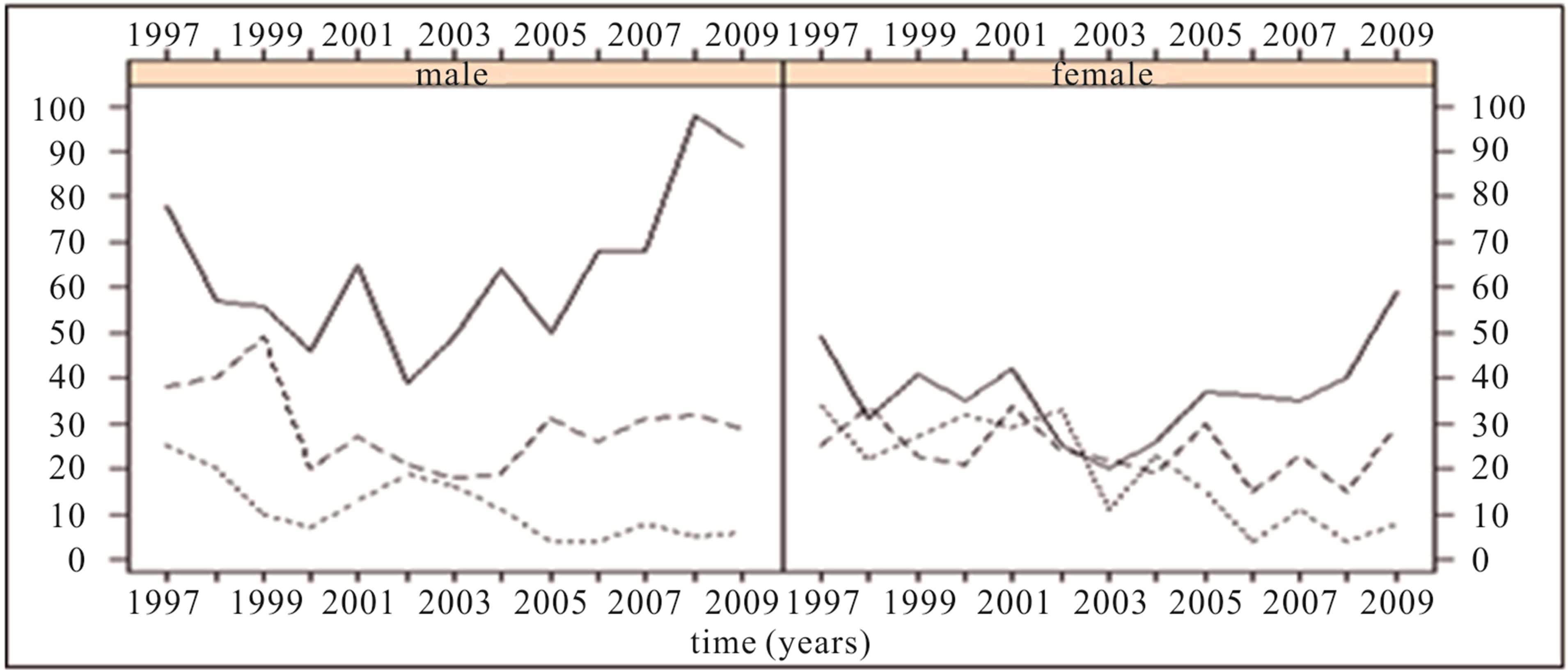
In Figures 2(a) to (c), we display readmissions, stratified by age and gender, as yearly counts, rates per 100,000 population and readmission rates, respectively. A close correspondence between counts and population rates for all age groups can be seen, however, similarity between population and readmission rates is present only for 2 - 5 year olds while the older age groups show a stark contrast. Although not shown here, regression analyses indicated a linear correspondence between counts and population rates but not between readmission rates and population rates.
3.1. Semi Parametric Models
We fitted our model to total readmissions and to male and female readmissions separately. The model showed that both month and day of the week had significant associations with mean daily readmission counts. Higher counts were expected in March, May, June and November, and the lowest counts in January. This pattern held for both males and females with males experiencing higher peaks. The day of the week had more of an impact for girls than boys. Overall more readmissions expected earlier in the week, from Sunday onwards, and the fewest on Saturday.
The fitted model produced a dispersion scaling parameter which was very close to unity, further justifying the assumption of a Poisson process and explaining why the negative binomial was such a bad fit. The smooth function of time was also significant (p < 0.0005), and indicated that after an initial trend of declining readmission counts until about 2001-2002, they subsequently began to increase returning to roughly initial levels (Figure 3).
Exploration with auto correlation plots and DurbinWatson tests indicated a weak but statistically significant auto correlation at lag 1 of 0.1, 0.08 and 0.06 for total, male and female readmissions respectively and so violated the assumption of independence of the daily readmission counts. In order to adjust for non independence, lag one values were included as part of the GAM. They made no substantial difference to the results and were finally not included due to the predictive role of our model.
3.2. Non Parametric Models
The non parametric model also demonstrated time, day of the week as well as day of year to be significantly associated with readmission counts. The day of year variable was in complete agreement with the parametric monthly variable of our final model for both timing and amplitude of peaks and troughs throughout the year.


Table 1. Distribution of counts of readmissions within 28 days for fiscal years 1997-2009.
 (a)
(a)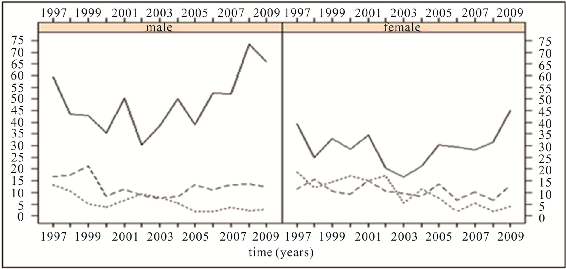 (b)
(b)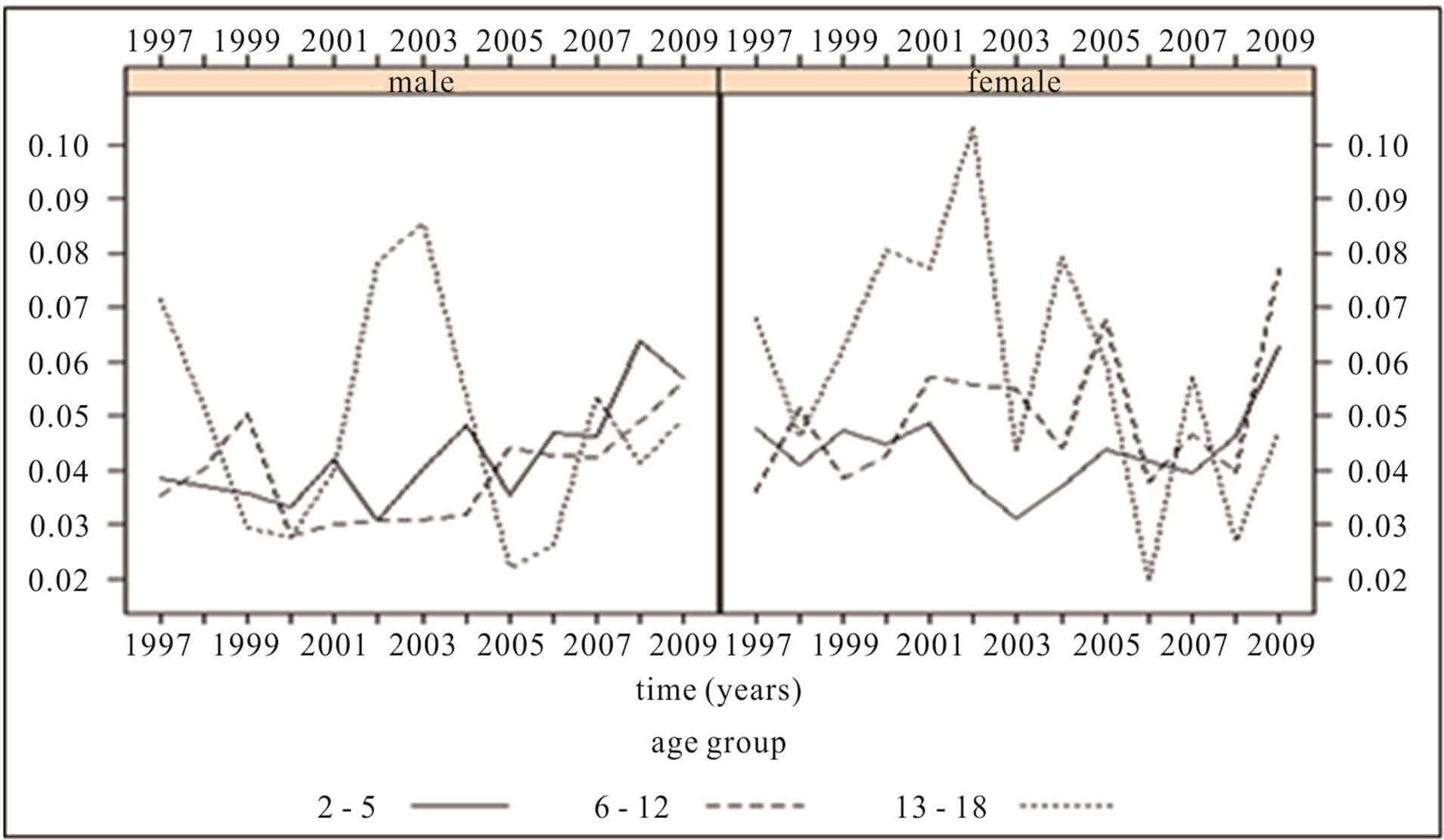 (c)
(c)
Figure 2. (a) Annual count of readmission within 28 days; (b) Annual rate of readmission within 28 days per 100,000 population; (c) Annual rate of readmission within 28 days per total number of admissions.
3.3. Model Validation
We validated the model predictions by training the model with the first 11 years of data then using the model to predict the final two years of data. The predictions were subsequently aggregated by month and compared to the actual data. χ2 goodness-of-fit tests indicated that there was no statistical difference between the predictions and the data (p = 0.65). In comparison, when using the mean of the training data as a predictor of the final 2 years of data, χ2 tests indicated that the monthly aggregated mean predictions were not a good fit to the data (p = 0.03). We also used this method to test the parametric model’s fit to the data and found very similar results to the semi parametric model’s but with slightly higher χ2 values and so the parametric model did not have as good a fit to the data as the semi parametric
 (a) Boys
 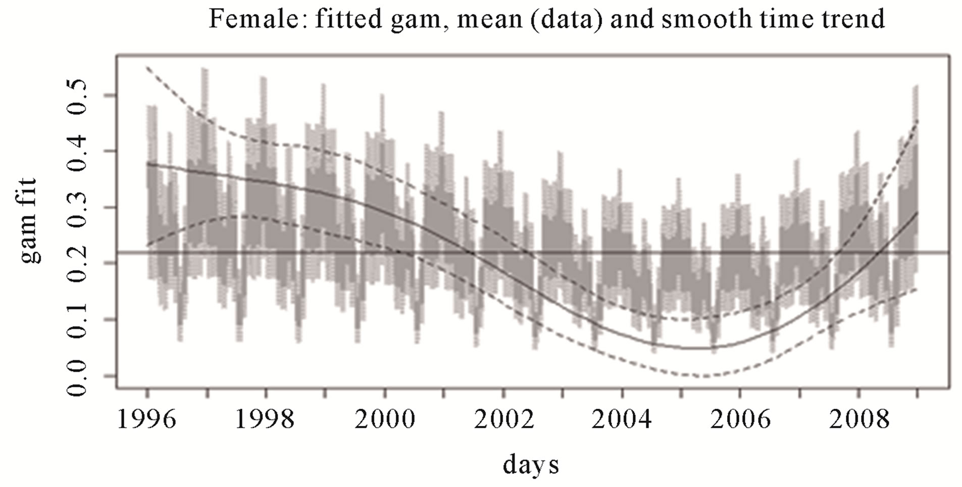 (b) Girls
Figure 3. Fitted semi parametric GAM and time trend to boys’ (a) and girls’ (b) daily readmission counts. Dotted lines represent 95% error limits. The horizontal lines are the overall means for the respective data subsets.
model. As the semi parametric model outperformed both the mean and the non parametric model in predicting the final 2 years of readmission data this gave us some confidence in using it to predict future readmissions.
Semi parametric models were also fitted to data subsets consisting of the 6 combinations of age group and sex displayed in Figure 2. Of these subsets, the largest number of total readmissions was for 2 to 5 year old boys, N = 829, and the smallest was for 13 to 18 year old girls, N = 253. In the presence of these extremely small numbers, the GAM was still sensitive to seasonality, day of the week and the time trend, with differences in the values of these covariates for the various subsets. The results of the χ2 goodness-of-fit tests validated the fit and prediction, but were only marginally better than the mean. Due to their extremely small numbers and the marginal improvement on the mean, we could not consider the models reliable for these 6 subsets.
Table 2 shows the actual data for 2009, in fortnightly aggregates, alongside the semi parametric GAM predictions for the same period. The data predictions were obtained with the same method used for model validation. The model was trained on the first 11 years of data and then used to predict the final two years of data. The predictions largely follow the previous year’s seasonal patterns, but with smoothed troughs and peaks. There are major differences in fortnights 18 & 19 and 25 & 26 representing March and June respectively. From Figure 1, we see that the March 2009 counts were unusually high and the June 2009 counts unusually low for those times of the year and so these differences may be due to normal variability or to the smoothing effect of the model. Table 2 shows that the confidence intervals for predictions after fortnight 17 tended to be the widest which indicated a decreasing reliability with an increasing predictive length. These predictions were for two years and so predictions of not more than one year are likely to be more reliable. However, overall, the predictions are in keeping with the seasonal character of the data.
3.4. Future Predictions
To obtain future predictions we trained the model on the
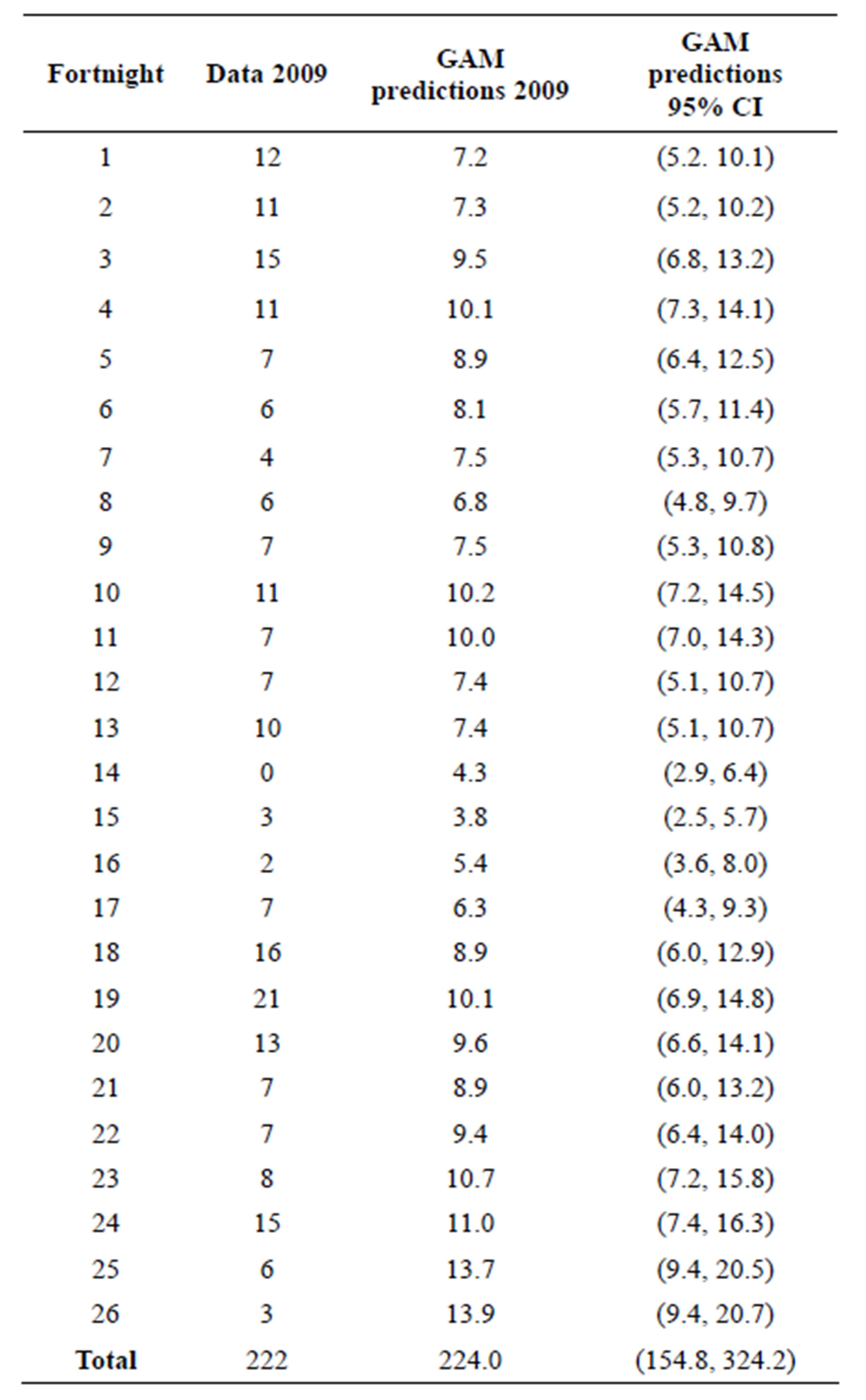
Table 2. Total readmissions within 28 days, in fortnight aggregates, for 2009 are compared to semi parametric GAM predictions with a 95% CI for the same period.
full 13 years of data and then predicted 12 months ahead.
In Figure 4, we graphed the predicted readmissions one year after study end. The predictions largely follow the previous year’s seasonal patterns, but with smoothed troughs and peaks. As with the 2009 data predictions, there are differences in June and in March probably due to the same factors as explained in the validation section. The predictions are similar with respect to seasonal patterns but they also suggest an increasing trend in readmissions. The predictions indicate that readmissions will continue to grow by up to 5% a year on average overall. Although not shown here, time trends for each of the three age groups indicated that the youngest age group, that is 2 - 5 years, will experience the largest increase and especially the boys.
4. DISCUSSION
This study is the first to predict childhood asthma hospital readmission counts using a semi-parametric generalized additive model. The model suggested an increasing time trend in readmission counts from about 2003-2004 to study end in June 2009, and indicated that certain months of the year and days of the week were more likely to register higher readmissions. The model’s predictions suggested that this increasing trend continued into the year after the end of the study. The total forecasts for 2010 suggest a return close to the high yearly totals at the commencement of the study. Even the lowest point of the 95% CI for the 2010 prediction is in keeping with this increasing trend.
To the best of our knowledge, only one other study has used time series methods to examine paediatric asthma readmissions [23]. The authors used Holt’s method, a weighting scheme for univariate time series with a linear trend [31], but did not report the method’s capacity for predictions. Annual readmission rates were their focus, and therefore their examinations of seasonality and day of the week were limited. The semi-parametric GAM approach has been recommended as a means of adjusting for any confounding associations of seasonality or day of the week in studies of air pollution and weather factors and daily counts of deaths or respiratory hospital admissions [32,33]. It has also been used both for this purpose [20] and to model seasonality [21] for paediatric hospital admissions. However, although none of these studies had produced predictions, they indicated GAM’s utility in modeling seasonality and day of the week associations with respiratory hospital admissions.
4.1. Comparisons to Admissions
Although Lincoln and colleagues [21] investigated admissions and not readmissions, their study is comparable to ours due to the mutual focus on seasonality and day of

Figure 4. Cumulative fortnightly predictions for 1 year after study end (2010) compared to the final study year (2009).
the week, some overlap with the study period (they used data from the period 1994-2000) and the Australian setting—Sydney, New South Wales (NSW). Lincoln and colleagues [21] also found, similarly to our study, that there tended to be greater numbers of admissions earlier in the week from Sunday onwards. The day of week association is likely an artefact of population interface with the Australian medical system rather than an intrinsic feature of asthma exacerbation. Choice of week end or week start is quite arbitrary. General practitioners are less likely to be available on weekends and perhaps parents hope children will improve with rest over the weekend. However, it is important to adjust for it so as to tease out any latent time trends and seasonality in daily data [28].
In the two studies, peaks in admissions and readmissions occurred at almost identical times of the year. The main difference in timing was with the May/June peak in readmissions. May/June corresponded with weeks 18 - 24. The Lincoln study [21] had an admission peak in June but in weeks 20 - 22 and not in May. The striking difference with these peaks concerned the relative amplitudes. The risk for admissions in the August peak did not reach statistical significance. However for readmissions we found that the May/June peak was far greater and more sustained than the other three peaks and, compared to March, the August peak was slightly higher and the November peak slightly lower. Furthermore, the November readmissions peak was high for boys but low for girls. Why should admission and readmission peaks coincide? Perhaps they reflect differences in timing of seasonal influences due to location and time of study. A weekly analysis, for comparison purposes, showed that weekly readmission in 28 days rates can be as high as 21% with IQR (2.7%, 4.2%, 6.5%). Lincoln and colleagues [21] did not differentiate admissions or readmissions within 28 days and so readmissions may have significantly augmented admission peaks. If this is so, the children who readmitted within 28 days displayed a greater and more sustained sensitivity to possible seasonal influences and experienced exacerbations earlier and more often. Our data also showed that, of the children who experienced a readmission within 28 days, 9% of them experienced another within the same 28 days.
4.2. Further Modeling Techniques
Artificial neural networks have been used to predict paediatric asthma admissions in Baltimore, USA [15] and Athens, Greece [16] . This approach produced accurate predictions of admissions, but due to the nature of this technique, it was not able to statistically assess seasonal, day of the week and time trend associations. Both studies predicted only one week ahead and neither provided long term predictions as have we. The Greek study ran over 4 years, 2001-2004, and considered age groups but not sex. The US study examined 14 years of data between 1986 and 1999 and considered age group, sex, ethnicity and compared the city of Baltimore to the rest of the state. Both studies described differences in frequencies of admissions based on seasonality, age group and sex which are similar to our findings. However, the authors of the Greek study noted that their approach was not reliable for the smaller numbers in the 5 - 14 age group. Given that the numbers of daily admissions for this group were far in excess of the numbers of total readmissions for our study, artificial neural networks may not be reliable for modeling low counts.
4.3. Strengths
Our study has a number of strengths. Firstly, our model was based on a large and comprehensive database that included all paediatric admissions for all Victorian public and private acute hospitals for the fiscal years 1997-2009. While admission criteria may vary both within and between hospitals, this has the potential to introduce random error which would push our estimates towards the null. Although we were modeling a low count time series, the length of the study period provided sufficient power to train our model and extend it into the future. Our model was sensitive to the seasonality, day of the week and time trend aspects of hospital readmissions. It achieved this in the presence of very low counts, even when the counts were reduced due to stratification by age group and sex. It was also sufficiently flexible to be able to reliably forecast readmission counts at fortnightly and monthly windows and can be extended for up to a year with these time frames. In forecasting future counts, the model showed itself robust to past outlier counts. Our method provided a way of modeling intrinsically difficult low count time series which may also prove useful in other settings besides child hospital asthma readmissions.
Previous studies examining the modeling of time series counts have compiled a check list of desired model features: flexibility to incorporate pronounced dependence structures in the data; ability to account for any overdispersion; easy to use link functions allowing for easy inference of covariate parameters; procedures for model fitting; diagnostic tools for assessing model adequacy; ease of forecasting [28,34]. Our model possessed these features further displaying its potential to be successfully applied in other settings. Furthermore, the semi parametric and fully parametric methods applied here, can be used respectively for parameter or observation driven models as categorised by Jung et al. [34]. It has been demonstrated that GAM computational methods may not be able to adjust for covariate correlation due to a back-fitting approach. This would result in low coefficient standard errors and therefore unreliably low p-values [35]. However, this does not apply to our model as the R package we used does not use back-fitting but instead fits penalized regression splines at once thus making the reliable calculation of the standard errors of the coefficient covariances possible [29]. This gives us confidence in the associations with season, day of the week and time trend detected by our model.
4.4. Limitations
One limitation of the study is that, once we assumed that seasonality is a marker for total environmental load, we could not differentiate between the various components of the environment such as weather, pollution, allergens and viral infections that may be associated with child asthma readmissions. However, the strong seasonal component in readmissions, indicated by our model, demonstrated the importance of the environment and showed that seasonal timing would be a good place to start an investigation of possible asthma exacerbation triggers. Although our model did not produce predictions on a hospital or area basis, it can still assist planning by health services and clinical management by indicating when adjustments to current management practices could be considered.
The predictive function of our model assumed a linear extrapolation into the future. This assumption may be good enough in the short term but may not hold for very long term predictions. However, 13 years of data gave us some reason to expect the not too distant future to be similar. At the very least, our model has the capacity to be updated or refined as new data come to hand. This model does not take individual risk factors into account but is still useful on an individual basis in that an individual who is prone to asthma exacerbations can be alerted beforehand of periods of a higher overall risk.
4.5. Conclusion
We have provided a reliable way of modeling low count time series such as daily childhood asthma hospital readmissions. Our model showed: there had been a strong seasonal impact on child asthma hospital readmissions; an increasing trend in readmissions until June, 2009; readmissions would continue to increase by up to 5% per year on average overall, with the 2 - 5 years age group experiencing the largest increase, especially for boys. This implies: clinical services may need to revise procedures and be alerted to possible greater risk of readmission at certain times of the year, especially for younger age groups; health services management may need to adjust resource allocation and planning.
REFERENCES
- Australian Centre for Asthma Monitoring. (2009) Asthma in Australian children: Findings from growing up in Australia, the longitudinal study of Australian children. AIHW, Canberra.
- Australian Centre for Asthma Monitoring. (2008) Asthma in Australia. AIHW, Canberra.
- Vollmer, W.M., Osborne, M.L. and Buist, A.S. (1993) Temporal trends in hospital-based episodes of asthma care in a health maintenance organization. American Review of Respiratory Disease, 147, 347-353. doi:10.1164/ajrccm/147.2.347
- Berry, J.G., Hall, D.E., Kuo, D.Z., Cohen, E., Agrawal, R., Feudtner, C., Hall, M., Kueser, J., Kaplan, W. and Neff, J. (2011) Hospital utilization and characteristics of patients experiencing recurrent readmissions within children’s hospitals. The Journal of the American Medical Association, 305, 682-690. doi:10.1001/jama.2011.122
- Watson, L., Turk, F. and Rabe, K.F. (2007) Burden of asthma in the hospital setting: An Australian analysis. International Journal of Clinical Practice, 61, 1884-1888. doi:10.1111/j.1742-1241.2007.01559.x
- McCaul, K.A., Wakefield, M.A., Roder, D.M., Ruffin, R.E., Heard, A.R., Alpers, J.H. and Staugas, R.E. (2000) Trends in hospital readmission for asthma: Has the Australian national asthma campaign had an effect? Medical Journal of Australia, 172, 62-66.
- Murray, C.S., Poletti, G., Kebadze, T., Morris, J., Woodcock, A., Johnston, S.L. and Custovic, A. (2006) Study of modifiable risk factors for asthma exacerbations: Virus infection and allergen exposure increase the risk of asthma hospital admissions in children. Thorax, 61, 376-382. doi:10.1136/thx.2005.042523
- Feudtner, C., Levin, J.E., Srivastava, R., Goodman, D.M., Slonim, A.D., Sharma, V., Shah, S.S., Pati, S., Fargason Jr., C. and Hall, M. (2009) How well can hospital readmission be predicted in a cohort of hospitalized children? A retrospective, multicenter study. Pediatrics, 123, 286- 293. doi:10.1542/peds.2007-3395
- Bloomberg, G.R., Trinkaus, K.M., Fisher Jr., E.B., Musick, J.R. and Strunk, R.C. (2003) Hospital readmissions for childhood asthma: A 10-year metropolitan study. American Journal of Respiratory and Critical Care Medicine, 167, 1068-1076. doi:10.1164/rccm.2201015
- Raymond, D., Henry, R.L., Higginbotham, N. and Coory, M. (1998) Predicting readmission to hospital with asthma. Journal of Paediatrics and Child Health, 34, 534-538. doi:10.1046/j.1440-1754.1998.00297.x
- Rasmussen, F., Taylor, D.R., Flannery, E.M., Cowan, J.O., Greene, J.M., Herbison, G.P. and Sears, M.R. (2002) Risk factors for hospital admission for asthma from childhood to young adulthood: A longitudinal population study. Journal of Allergy & Clinical Immunology, 110, 220-227. doi:10.1067/mai.2002.125295
- Alshehri, M., Almegamesi, T. and Alfrayh, A. (2004) Predictors of short-term readmission of asthmetic children. Journal of the Egyptian Public Health Association, 79, 165-178.
- Reznik, M., Hailpern, S.M. and Ozuah, P.O. (2006) Predictors of early hospital readmission for asthma among inner-city children. Journal of Asthma, 43, 37-40. doi:10.1080/02770900500446997
- Gorelick, M., Scribano, P.V., Stevens, M.W., Schultz, T. and Shults, J. (2008) Predicting need for hospitalization in acute pediatric asthma. Pediatric Emergency Care, 24, 735-744. doi:10.1097/PEC.0b013e31818c268f
- Blaisdell, C.J., Weiss, S.R., Kimes, D.S., Levine, E.R., Myers, M., Timmins, S. and Bollinger, M.E. (2002) Using seasonal variations in asthma hospitalizations in children to predict hospitalization frequency. Journal of Asthma, 39, 567-575. doi:10.1081/JAS-120014921
- Moustris, K.P., Douros, K., Nastos, P.T., Larissi, I.K., Anthracopoulos, M.B., Paliatsos, A.G. and Priftis, K.N. (2011) Seven-days-ahead forecasting of childhood asthma admissions using artificial neural networks in Athens, Greece. International Journal of Environmental Health Research, 22, 93-104. doi:10.1080/09603123.2011.605876
- Dales, R.E., Schweitzer, I., Toogood, J.H., Drouin, M., Yang, W., Dolovich, J. and Boulet, J. (1996) Respiratory infections and the autumn increase in asthma morbidity. European Respiratory Journal, 9, 72-77. doi:10.1183/09031936.96.09010072
- Fleming, D.M., Cross, K.W., Sunderland, R. and Ross, A.M. (2000) Comparison of the seasonal patterns of asthma identified in general practitioner episodes, hospital admissions, and deaths. Thorax, 55, 662-665. doi:10.1136/thorax.55.8.662
- Wong, G.W., Ko, F.W., Lau, T.S., Li, S.T., Hui, D., Pang, S.W., Leung, R., Fok, T.F. and Lai, C.K. (2001) Temporal relationship between air pollution and hospital admissions for asthmatic children in Hong Kong. Clinical & Experimental Allergy, 31, 565-569. doi:10.1046/j.1365-2222.2001.01063.x
- Lee, S.L., Wong, W.H. and Lau, Y.L. (2006) Association between air pollution and asthma admission among children in Hong Kong. Clinical & Experimental Allergy, 36, 1138-1146. doi:10.1111/j.1365-2222.2006.02555.x
- Lincoln, D., Morgan, G., Sheppeard, V., Jalaludin, B., Corbett, S. and Beard, J. (2006) Childhood asthma and return to school in Sydney, Australia. Public Health, 120, 854-862. doi:10.1016/j.puhe.2006.05.015
- Sears, M.R. and Johnston, N.W. (2007) Understanding the September asthma epidemic. Journal of Allergy and Clinical Immunology, 120, 526-529. doi:10.1016/j.jaci.2007.05.047
- Jonasson, G., Lodrup Carlsen, K.C., Leegaard, J., Carlsen, K.H., Mowinckel, P. and Halvorsen, K.S. (2000) Trends in hospital admissions for childhood asthma in Oslo, Norway, 1980-95. Allergy, 55, 232-239. doi:10.1034/j.1398-9995.2000.00387.x
- Hastie, T. and Tibshirani, R. (1986) Generalized additive models. Statistical Science, 1, 297-310.
- Vicendese, D., Abramson, M.J., Dharmage, S.C., Tang, M.L., Allen, K.J. and Erbas, B. (2012) The influence of age, gender and seasonality on asthma readmissions among children and adolescents over time. LaTrobe University, Bundoora.
- Chambers, M. and Clarke, A. (1990) Measuring readmission rates. British Medical Journal, 301, 1134-1136. doi:10.1136/bmj.301.6761.1134
- Ashton, C.M., Del Junco, D.J., Souchek, J., Wray, N.P. and Mansyur, C.L. (1997) The association between the quality of inpatient care and early readmission: A metaanalysis of the evidence. Medical Care, 35, 1044-1059. doi:10.1097/00005650-199710000-00006
- Davis, R.A., Dunsmuir, W.T.M. and Wang, Y. (1980) Modelling Time Series of Count Data.
- Wood, S.N. (2006) Generalised additive models—An Introduction with R. Chapman & Hall/CRC. Taylor & Francis Group.
- Sarkar, D. (2008) Lattice: Multivariate data visualization with R. Springer, New York.
- Hyndman, R.J. and Athanasopoulos, G. (2012) Forecasting: Principles and practice. http://otexts.com/fpp/7/2/
- Schwartz, J. (1994) Nonparametric smoothing in the analysis of air pollution and respiratory illness. Canadian Journal of Statistics, 22, 471-487. doi:10.2307/3315405
- Katsouyanni, K., Touloumi, G., Samoli, E., Gryparis, A., Le Tertre, A., Monopolis, Y., Rossi, G., Zmirou, D., Ballester, F., Boumghar, A., Anderson, H.R., Wojtyniak, B., Paldy, A., Braunstein, R., Pekkanen, J., Schindler, C. and Schwartz, J. (2001) Confounding and effect modification in the short-term effects of ambient particles on total mortality: Results from 29 European cities within the APHEA2 project. Epidemiology, 12, 521-531. doi:10.1097/00001648-200109000-00011
- Jung, R.C., Kukuk, M. and Liesenfeld, R. (2006) Time series of count data: Modeling, estimation and diagnostics. Computational Statistics & Data Analysis, 51, 2350-2364. doi:10.1016/j.csda.2006.08.001
- Dominici, F., McDermott, A., Zeger, S.L. and Samet, J.M. (2002) On the use of generalized additive models in timeseries studies of air pollution and health. American Journal of Epidemiology, 156, 193-203. doi:10.1093/aje/kwf062
NOTES
*Corresponding author.