Open Journal of Civil Engineering
Vol.3 No.1(2013), Article ID:29468,10 pages DOI:10.4236/ojce.2013.31004
New System of Structural Health Monitoring
School of Engineering, University of North Florida, Jacksonville, USA
Email: ahmed.gamal@unf.edu, adel.el-safty@unf.edu, gmerckel@unf.edu
Received November 20, 2012; revised December 30, 2012; accepted January 5, 2013
Keywords: Health Monitoring; Wireless; Cellular; Data Processing; Structures
ABSTRACT
Monitoring of structures is an important challenge faced by researchers worldwide. This study developed a new structural health monitoring system which utilized the use of microprocessors, wireless communication, transducer, and cellular transmission that allows remote monitoring. The developed system will facilitate the monitoring process at any time and in any location with less human interference. The system is equipped with data processing subsystem which works on detection of structural behavior irregularity, defects, and potential failures. The system was tested using strain gages to measure the developed strains in different applications and structural models. The results developed using the new system showed that the generated readings from the system followed correctly the expected trend according to structural concepts. The developed system accomplished the desired features of lower cost, less power, reduced size, flexibility and easier implementation, remote accessing, early detection of problems, and simplified representation of the results.
1. Introduction
In the United States, 50% of all bridges were built before 1940s, and approximately 42% of these structures are structurally deficient [1]. It has been estimated that the investments needed to enhance the performance of deficient structures exceed $900 billion worldwide. These statistics show the importance of developing new techniques of measuring the health of structural with less manual effort and hence less mistakes. In 2007, the collapse of Minnesota Bridge over Mississippi river attracted the attention to the need of giving more attention to the safety of infrastructure issues across the whole country.
In 1990, the Minnesota Bridge was issued a certificate of “structurally deficient” due to significant corrosion in the bearings, and the bridge was repaired. In 2005 and 2006, the Minnesota department of transportation’s engineers inspected the bridge visually and made a report about the condition of the bridge [2]. After the collapse, the bridge was reconstructed and instrumented with smart health monitoring systems. Approximately four different kinds of sensors were used: accelerometers, chloride penetration sensor, linear potentiometers, and wire strain gauges. All the sensors are wired using fiber optics where data collected are wirelessly transmitted to be correlated with design codes to analyze the performance of the bridge over its life span. The main challenges facing structural health monitoring in Minnesota Bridge are the difficulty to pinpoint what is happening in a specific location, to lower the cost of the system, and to reduce the power consumption.
New systems of structural health monitoring have been developed with different approaches such as using wireless sensors with self-diagnosing and self-calibration to reduce data transmission, thus reducing power consumption [3]. Other systems implemented wireless sensors which are capable of actuation, in which the sensor node is able to fix the problems detected without sending the data to the control node so that the power used can be reduced [4]. A different approach is based on covering the structures with piezoelectric layer and sending mechanical impedance through the layer and then measuring the electrical impedance of the layer [5]. Power consumption is a major problem in structural health monitoring. Many researchers tried to overcome this problem by different techniques such as solar and wind energy, self-acquisition of sensors, and sensors actuation. Other improvements investigated and recommended in those researches are reducing the size of the system, increasing the read range, more memory, and improving the ruggedness and robustness of the sensor node.
Based on previous studies, most of the problems facing structures’ health occur due to excessive strain, corrosion, temperature changes, or fatigue. Any abnormal increase in strains and stresses or initiation of cracks in the structures should be detected. New monitoring systems for the health of the structures need to be developed to utilize the advances in the microprocessors and communication technologies. The new system should have the following specifications:
1) Low cost and low energy consumption.
2) Remote accessing.
3) High speed communication.
4) Real time identification of the problems.
5) Simplified representation of the results.
6) Disaster patterns for early identifications of problem.
7) Less space and easier implementation.
The monitoring system is designed to monitor the main parameters affecting the health of structures in general and bridges in specific. Through looking for changes in parameters that are sensitive to the change, an estimate of the overall health of a system can be reached [6]. The new developed system in this study can be used to monitor strain, deflection, temperature, and corrosion.
2. Experimental Setup
The experimental setup was divided into four different stages to address different aspects with more accurate interpretation. The four stages of the experimental setup are:
1) Sensor node and sensor implementation (instrumentation of structural members);
2) Data transmission;
3) Data processing;
4) Data presentation.
Sensor node and sensor implementation: The main objective of this stage is to reduce the size of the sensor node which allows easier implementation of the node in any location of the structure. In this stage, the focus was directed towards integrating electrical engineering with civil engineering concepts in order to achieve the desired outcome. The main factor that the sensor node was based on was using the advanced technology in microprocessor. In this sensor node, the transducer was attached to the microprocessor through interface circuit which permits necessary functions through less size and time while increasing the accuracy of the output. The interface circuit aims to collect and amplify the output from the transducer and feed this output to the input of analog-to-digital convertor (ADC). The ADC converts the transducer readings to digital readings in order to be processed and transmitted by the microprocessor. The interface circuit contains a differential circuit followed by an amplification circuit, Figure 1.
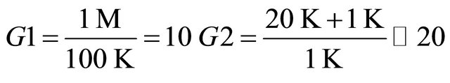
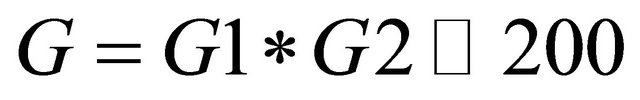
The differential circuit is represented by a differential amplifier that has a gain equals to
 (1)
(1)
while the amplifying circuit is composed of a non-inverting amplifier with gain equals to
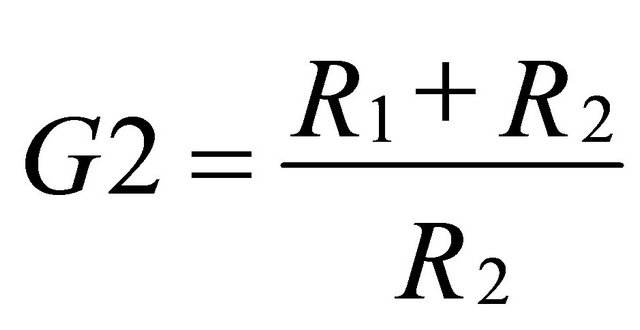 (2)
(2)
The output from the amplification circuit is fed to the input pin of the ADC which converts the input to digital output as shown in the following equation, The output from the ADC is stored in the memory registers located on the microprocessor board to be processed and transmitted.
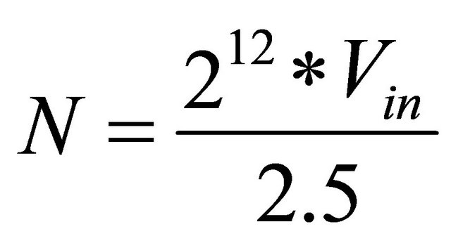 (3)
(3)
Each sensor node consists of central processing unit (CPU) represented by the microprocessor (e.g. MSP430- F6137), Figure 2, connected to the analog-to-digital converter (ADC). The readings from the transducer go through the conversion cycle while it is compared to the predefined threshold values through the comparator found in the CPU. In case of any irregularity, the RF antenna located on the microprocessor board receives an interrupt (alarming message) from the CPU to send a warning message to the main control unit for immediate action.
Two different setups were constructed to implement the sensor nodes in order to test the new system. The first structure was composed of a steel plate supported on two wooden blocks which was used as preliminary setup to test strain gages and Linear Variable Differential Transformer LVDT through flexural bending under three-point loading, Figure 3. The second setup was a small-scale
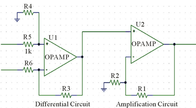
Figure 1. Interface circuit schematic.
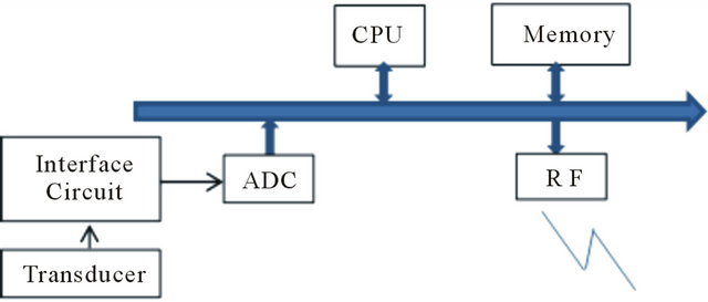
Figure 2. Typical sensor diagram.
bridge composed of interconnected truss members. The truss bridge was loaded with stationary and moving loads, Figure 4. This bridge setup was used to verify the preliminary readings gathered from the first setup of steel plate structure through bending of the bridge track/deck as well as testing the axial strains developed in the truss bridge members.
Data transmission: The second stage after data collection on the sensor node was transmitting these data to different part of the system. To optimize the transmission, the system was divided into three subsystems, as shown in Figure 5. The first subsystem was composed of the sensor nodes which were connected directly to different members of the structure. The second subsystem which is the main control unit is connected to the sensor nodes subsystems through wireless communication. The third subsystem which represents the final stage for the data represents the monitor unit. The monitor unit is connected to the main control unit through cellular data transmission.
The control unit acts as a link between the measuring device and the end user, and also acts as the brain of the entire system. The second subsystem consists of a microprocessor (e.g. MSP430) connected to the RF transmission unit, and cellular transmission unit. The control unit is the intermediate stage which is responsible of
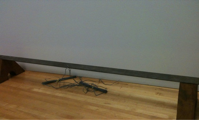
Figure 3. Steel bar setup.

Figure 4. Bridge setup.
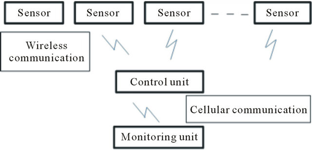
Figure 5. System design.
conveying data from the sensors node to the monitor unit, as well as carrying commands from and into the sensors node and from and into the monitor unit. The control unit stays in a low power mode until it is activated by the sensor node or the monitor unit to save power. When the control unit is activated, the cellular transmission unit and RF transmission unit are activated in order to receive data from the sensor node and send it to the monitor unit, or to receive commands from the monitor unit and send them to the sensor node.
The monitor unit is the user interface, where represents the final destination of the data collected. The monitor unit’s responsibility is to receive commands from the user and send them to the control unit as well as receiving data from the control unit. The monitor unit is composed of software development kit. The software is webbased program responsible for collecting, processing, and displaying the data in a graphical representation. In addition, the software alerts the user when any exception or irregularity takes place in the data collected.
To ensure a proper secured transmission of the correct message, a communication protocol was defined. This protocol is recognized by the sending and the receiving end. The protocol represents the conversation between the two ends to verify the complete transmission of the correct message. The communication starts when the sending end collects necessary information about the message to be sent. The message is sent with its information to the transmitting end of the RF transmission channel. The transmitting end sends a sending acknowledgement to the receiving end. When the receiving end receives the acknowledgement, the transmitting end starts to send the information about the message followed by the message itself. Once the complete message is received, Cyclic Redundancy Check (CRC) register checks the message received to verify that the correct message is received. After verifying receiving the correct message, an acknowledgement message is sent back to the transmitting end. When a wrong or incomplete message is sent or no acknowledgement is received from the other end, the transmission end restarts the transmission of the data. This step is repeated for three times. If the same situation continues after the third time, the transmitting end sends an error report to the CPU which calls for immediate action. The flow chart for the transmission protocol is shown in Figure 6.
The packet structure represents the structure of the message being sent between the transmitting end and the receiving end. The message is divided into four parts; each one carries certain information about the message. Each part of the message is a multiply of a byte long. Figure 7 shows the packet structure.
Each part of the message is defined as follows:
1) Sender and Receiver (S/R) Address: 1 Byte indicates the address of the sender node and the receiving node with the most significant bit (MSB) reserved for address extension for more nodes to be connected.
Example of node address:
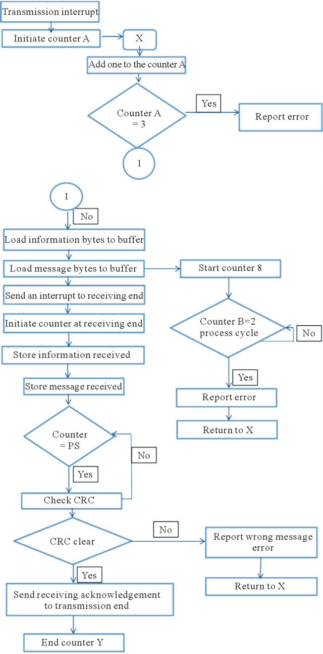
Figure 6. Transmission protocol flowcharts.
0001: Control unit.
0010: Sensor 1/unit 1.
0011: Sensor 2/unit 1.
0100: Sensor 3/unit 1.
Identity byte: 1 Byte contains the necessary information to identify the transmitted message. It includes 1 bit for priority (error), 1 bit as initiator to indicate the presence of data message attached to the message being sent, and packet size. In case an error is being sent, no data can be sent at the same time in Table 1.
2) Command/Error a) Error byte: The error byte indicates the presence of an error in any part of the system. Each bit in the error byte refers to a certain part of the system; the high state of this bit indicates the presence of an error in Figure 8.
b) Command byte: The command byte is always preceding the data bytes to identify the type of the data sent and any command need to be sent to the receiving end. The first four bits identify the type of data sent. Each measuring device is assigned one bit, and the high state of the bit indicates the data transmission from this device. If more than one device is activated at the same time, the data are transmitted according to the sequence of the devices, as follows: strain gages, LVDT, temperature sensor, and corrosion. The last four bits are reserved for the commands to be sent to the receiving end Figure 9.
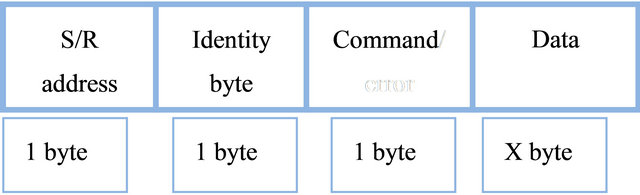
Figure 7. Packet structure.
Table 1. Identity byte examples.
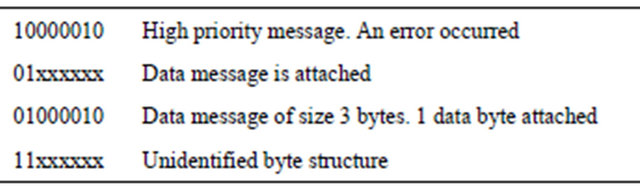
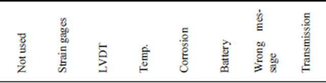
Figure 8. Error byte bits divisions.
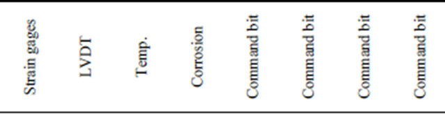
Figure 9. Command byte bit divisions.
IV-Data message: X bytes indicating the data message transmitted. The number of bytes of the message is identified from the packet size transmitted earlier. Each device is assigned one byte of data.
Data processing: When the data reach the monitor unit, the data go through data processing to reach the final format of the readings which can be presented to the end user. This data processing starts with digital-to-analog conversion which can be done using digital-to-analog convertor (DAC) located on the microprocessor board. The conversion is followed by voltage conversion cycles based on the parameters being measured. This conversion is discussed in the results section.
Data presentation: When the final format of the readings is reached, the readings are presented for review using graphical representations and table forms for easier interpretation. Data processing and data presentation can be conducted using MATLAB or any similar software. Those presentations are uploaded to a web-based database through MySQL or any similar software.
3. System Testing
In order to test the system, the system was assembled using strain gages as transducers to measure strain. The concept of Wheatstone bridge was used where the strain gage is used as one of the resistors in the bridge in case of using quarter bridge or two strain gages were used as two resistors in the bridge in different directions in case of using half bridge, Figure 10.
The interface circuit was assembled using the following resistors’ values, R5 = R6 = 120 kΩ, R7 = R8 = 1 MΩ, while R9 = 20 KΩ and R10 = 1 Ω. The gain was calculated as below:
 (4)
(4)
 (5)
(5)
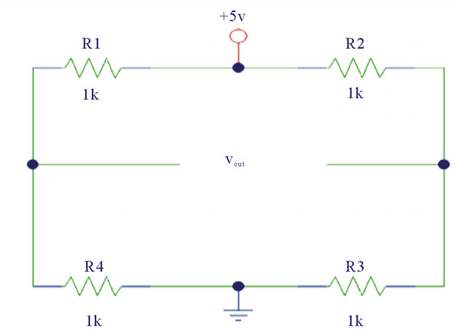
Figure 10. Wheatstone bridge schematic.
The entire circuit pictures and schematic are shown in Figures 11-14.
Three different types of tests were conducted to measure the efficiency of the system. In the first test, the strain gages were bonded to the steel plate top and bottom surfaces at mid span. The gages measured the developed bending strains in the steel plate that was subjected to 3-point loading (static flexural testing). The second test was conducted through bonding strain gages to the track of the truss bridge to measure the bending strains developed in the track/deck due to the movement of a truck load (dynamic testing). The third test was conducted by applying loads on the truss bridge and measure the tension strains developed in the bridge members by the attached strain gage (static testing). The voltage output from the circuit was recorded by the ADC where it con-

Figure 11. Full system schematic.

Figure 12. Work station.
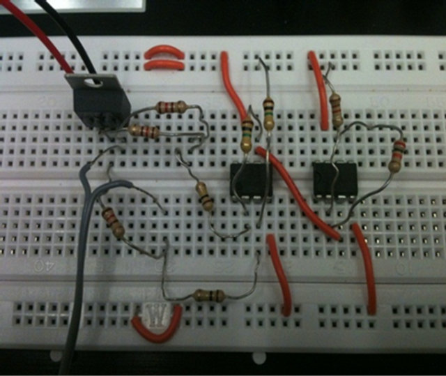
Figure 13. Full system circuit.
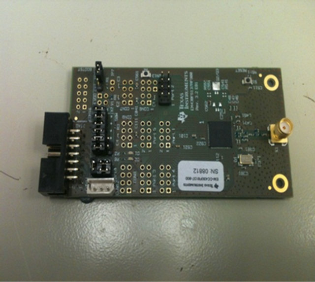
Figure 14. Microprocessor board.
verted it to digital values to be transmitted through RF antenna. The digital values were converted back to their original values. Then they were converted to their equivalent strain values through the following equations [7]:
For quarter bridge connection:
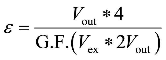 (6)
(6)
For half bridge connection:
 (7)
(7)
where  is strain, Vex is the supply voltage to the Wheatstone bridge, and G.F. is gage factor. In case of metal strain gages, G.F. is equal to 2.019. The strain values were stored and presented graphically for better interpretation of the data gathered and to ensure the efficiency of the system. The data conversion to strain values and graphical presentation were conducted through GUE-Octave which is equivalent to MATLAB but with open source for demonstration purposes.
4. Results and Analysis
a) First testing findings
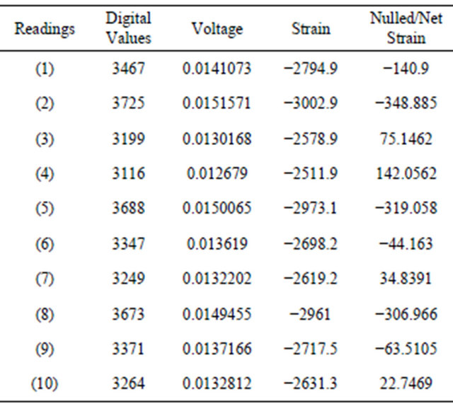
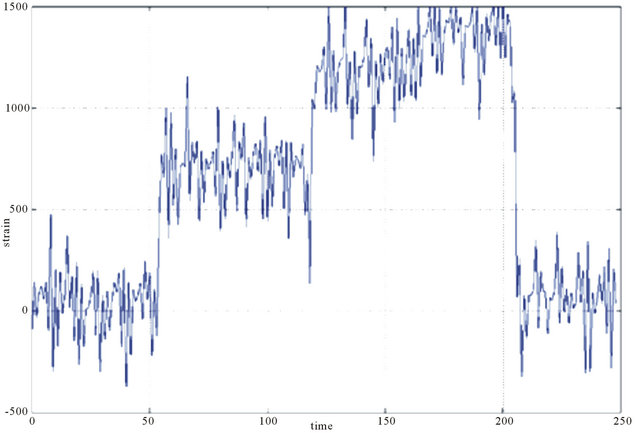
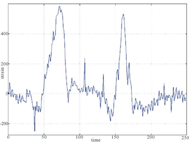
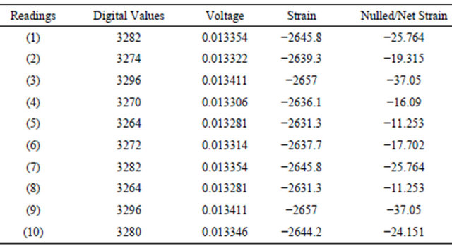
Through the first static test conducted on the steel plate structure, the procedures were conducted several times using half-bridge configuration. In each time, the voltage values are recorded as well as the strain values after conversion. The strain values are plotted versus time to show change in strain due to applying loads to the plate. The following tables represent some samples from the data gathered. Each table contains the digital values, voltage values, strain values, and nulled/net strain values, as shown in Table 2. The following figures represent the strain values associated with applying different loads. Figures 15(a) and (b) represent the change in strain due to applying increasing loads of different weights.
b) Second testing findings
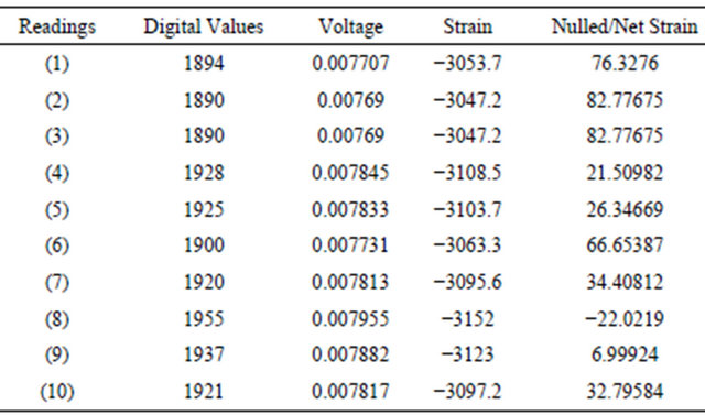
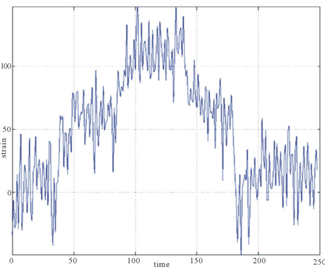
The second testing procedure represents the dynamic testing of the bridge deck using quarter bridge technique. This test was used to validate the results gathered in the first testing procedure and increase the credibility of the system. The testing was carried out by moving a loaded truck over the bridge track and measure the bending strain developed in the track/deck. The measuring procedure was repeated several times. Table 3 represents the recorded values as explained in the first testing findings. The following figures represent the recorded strains during moving the loaded truck. Figure 16(a) shows the change in strain when passing the truck twice on the bridge.
Table 2. First testing values.
 (a)
(a) (b)
(b)
Figure 15. First testing strain graphs: (a) Adding two similar loads consecutively; (b) Adding one load towards the end.
Table 3. Second testing values.
 (a)
(a) (b)
(b)
Figure 16. Second testing strain graphs: (a) Passing the truck twice; (b) Passing the car three times.
Figure 16(b) shows the changes when passing the truck three times.
c) Third testing findings
The third testing is considered a static test conducted on the truss bridge member using half bridge technique. The tensile strains developed in the bridge truss members were measured to test the efficiency of this system in different application. Table 4 represents samples from the recorded data as mentioned in the previous tests. The following figure represents the change in tensile strain readings by applying different loads to the bridge. Figure 17 shows the increase in tensile strains due to increasing the applied loads and the decrease upon removing the loads.
Testing the system using strain gages to measure strain in different applications ensures the efficiency of the system. The results developed using the new system showed that the generated readings from the system followed correctly the expected trend according to mechanics and structural analysis concepts. The results showed that the strains increased when increasing the applied loads, within the estimated range.
5. Conclusions
After specifying the required features of the new system for structural health monitoring, the system design and architecture were developed to serve those features. Using the microprocessor with the attached ADC and memory enabled the sensor node to store and process data, which reduces the transmission between the different parts. This reduction in the data transmission will reduce the power consumed by the system. The cellular transmission allows instant access to the data from any
Table 4. Third testing values.
 (a)
(a)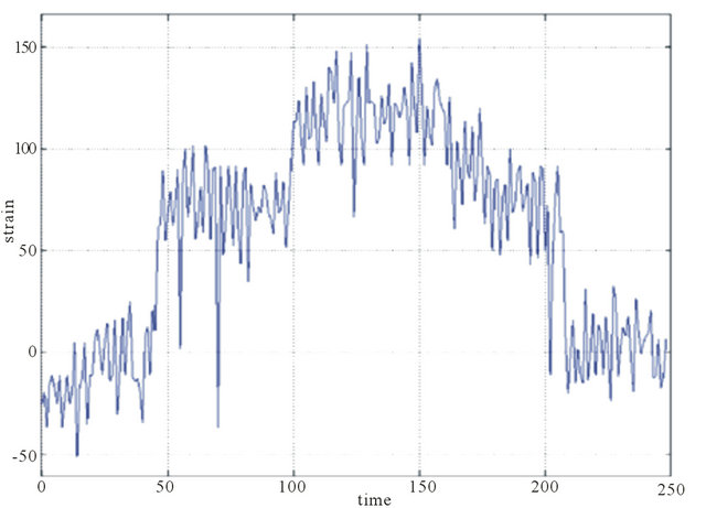 (b)
(b)
Figure 17. Third Testing strain graphs: (a) Adding two similar loads consecutively; (b) Adding two similar loads consecutively.
location. The system architecture was developed to serve the purpose of secured and reliable transmission. The communication protocol ensures the acknowledgment of receiving the correct message by the receiving end. The packet structure was formed in a specific form to add the advantage of having variable message length of different types such as data message, command message, or error message.
The system is powered through solar energy which ensures a reliable source of energy. This solar energy will lower the costs of the system when considering the long term application. Using the developed electrical circuits to replace the traditional data acquisition systems will reduce the overall cost. These electrical circuits connected to the microprocessor reduced the overall size of the system and facilitate the application of the system in any location.
Testing the system through using strain gages showed the efficiency of the tests and its operation in different applications. The same system can be applied to different transducers with minor modifications. The main idea of the system depends on recording an output voltage from the transducer in order to apply it to the microprocessor. The developed system in this study accomplished the desired features of lower cost, less power, reduced size, flexibility and easier implementation, remote accessing, early detection of problems, and simplified representation of the results. This will help minimizing the chances of structural collapses.
REFERENCES
- F. W. Klaiber, K. F. Dunker, T. J. Wipf and W. W. Sanders, “Methods of Strengthening Existing Highway Bridges,” NCHRP Rep. 293, Transportation Research Board, National Research Council, Washington DC, 1987.
- Minnesota Public Radio, “I-35W Bridge Fact Sheet,” 3 August 2007.
- B. F. Spencer Jr., M. E. Ruiz-Sandoval and N. Krata, “Smart Sensing Technology: Opportunities and Challenges,” Journal of Structural Control and Health Monitoring, Vol. 11, No. 4, 2004, pp. 349-368. doi:10.1002/stc.48
- J. P. Lynch and K. J. Loh, “A Summary Review of Wireless Sensors and Sensor Networks for Structural Health Monitoring,” Shock and Vibration Digest, Vol. 38, No. 2, 2006, pp. 91-128. doi:10.1177/0583102406061499
- D. L. Mascarenas, M. D. Todd, G. Park and C. R. Farrar, “Development of an Impedance Based Wire-Less Sensor for Structural Health Monitoring,” Smart Materials and Structures, Vol. 16, No. 6, 2007, pp. 2137-2145. doi:10.1088/0964-1726/16/6/016
- C. R. Bennett, A. Chamorro, C. Chen, H. Solminihac and G. W. Flintsch, “Data Collection Technologies for Road Management,” 2007, in press.
- National Instruments, “Strain Gauge Measurement—A Tutorial,” 1989.