Open Journal of Modern Hydrology
Vol.06 No.04(2016), Article ID:71371,23 pages
10.4236/ojmh.2016.64019
Application of the Reciprocal Analysis for Sensible and Latent Heat Fluxes with Evapotranspiration at a Humid Region
Toshisuke Maruyama*, Manabu Segawa
Faculty of Environmental Science, Ishikawa Prefectural University, Ishikawa, Japan

Copyright © 2016 by authors and Scientific Research Publishing Inc.
This work is licensed under the Creative Commons Attribution International License (CC BY 4.0).
http://creativecommons.org/licenses/by/4.0/


Received: August 17, 2016; Accepted: October 17, 2016; Published: October 20, 2016
ABSTRACT
Evapotranspiration acts an important role in hydrologic cycle and water resources planning. But the estimation issue still remains until nowadays. This research attempts to make clear this problem by the following way. In a humid region, by applying the Bowen ratio concept and optimum procedure on the soil surface, sensible and latent heat fluxes are estimated using net radiation (Rn) and heat flux into the ground (G). The method uses air temperature and humidity at a single height by reciprocally determining the soil surface temperature (Ts) and the relative humidity (rehs). This feature can be remarkably extended to the utilization. The validity of the method is confirmed by comparing of observed and estimated latent (lE) and sensible heat flux (H) using the eddy covariance method. The hourly change of the lE, H, Ts and rehs on the soil surface, yearly change of lE and H and relationship of estimated lE and H versus observed are clarified. Furthermore, monthly evapotranspiration is estimated from the lE. The research was conducted using hourly data of FLUXNET at a site of Japan, three sites of the United States and two sites of Europe in humid regions having over 1000 mm of annual precipitation.
Keywords:
Bowen Ratio, Eddy Covariance, Reciprocal Determination, Estimation of Sensible and Latent Heat Fluxes, Soil Surface Temperature and Humidity

1. Introduction
In the natural world, the air temperature and humidity are determined by H and lE from the net radiation (Rn) and heat flux into the ground (G). Therefore, our research attempts the reciprocal analysis of H and lE from the air temperature (Tz) and humidity (rehz) at single height while satisfying the heat balance relationship. The concept can’t find the other relevant methods, and it only requires Rn, G, Tz and rehz. This feature is remarkably widened a utilization purposes.
Recently, we reported the reciprocal analysis of sensible and latent heat fluxes in a forest region [1] . However, “humid region” is quite different from “forest region” because of no canopy. This paper described “humid region” instead of “forest region”, although there was similar concept in previous research.
The main different point is: the present paper contains two unknown variables, i.e., relative humidity (rehs) and temperature on the soil surface (Ts) while the previous paper contains only one variable, i.e., rehs, on the canopy surface. Therefore, the analysis has differences in that the present paper has to solve two simultaneous equations while the previous paper solved only one equation. In the analytical process, various new points arisen. Addition, this paper describes the comparison of the Penman method with our method because of humid region.
In the proposed method, the unknown variables, Ts and rehs were determined by the non-linear optimization technique known as the general reduced gradient (GRG) using the Excel Solver (Appendix 1).
2. Materials
We proposed a general method for estimating sensible and latent heat flux using single height temperature and humidity. The method contains two unknown variables: soil surface temperature, Ts, and humidity, rehs. This chapter describes the theoretical back- ground for estimating Ts and rehs, the practical procedure, data correction, the details of test sites and measurement instruments.
2.1. Method of Analysis
2.1.1. Fundamental Concept of the Model
A proposed model is somewhat similar to previous research [1] . Therefore, briefly the outline is described. The proposed model considers the near-soil surface as shown in Figure 1.

Figure 1. Components of the model and the relevant symbols.
Here, Rn is net radiation which is portioned into sensible, latent and underground heat fluxes. Ts is the soil surface temperature, Tz is the air temperature at height z,  is the specific moisture at height z, rehz is relative humidity in air at height z,
  is the unsaturated specific moisture on the soil surface, and
  is the saturated specific moisture on the soil surface.
The fundamental formulae of the model satisfy the following well-known heat balance relationship [2] .
 . (1)
. (1)
Here, Rn is the net radiation flux (W∙m−2), G is the heat flux into the ground (W∙m−2), H is the sensible heat flux (W∙m−2), and lE is the latent heat flux (W∙m−2).
In addition, the Bowen ratio (H/lE) is defined as follows [2] :
 . (2)
. (2)
We apply the concept of Bowen ratio to the layer between the soil surface and observation height of Tz and rehz. But, the Ts and  are just on the surface and usually unknown.
2.1.2. Governing Equation for Estimating the Unknown Variables Ts and rehs
The governing equation to be solved is obtained by heat balance relationship [1] . The unknown variables Ts and rehs are estimated as follows: The Ts and the , i.e., rehs × esat (Ts) are assumed initially; thus, the heat balance relationship has not closed as Equation (3):
 (3)
(3)
 (4)
(4)
 and
and . (5)
. (5)
Here i is number of iteration. Hest,i is estimated sensible heat flux in i times iteration, lEest,i is estimated latent heat flux, εi is residual of heat balance relationship of i times iteration, Tsass is assumed soil surface temperature,  is specific moisture at Tsass, Bapp is apparent ratio of sensible and latent heat flux under convergence process.
The approximated Ts and rehs putting in Equation (4), lE and H of next order approximated values obtained by Equation (5).
By repeating the above calculation from Equation (3) to Equation (5), the Bapp converged to B0 according to objective function ABS (εi) conversed to a minimum.
After optimization, Bapp is conversed to B0. Then, lEest and Hest can be obtained as follows:
 and
and . (6)
. (6)
To estimate Ts, an adjustment factor RTs was introduced using T0 as follows:
 . (7)
. (7)
Here, T0 is the observed soil temperature (˚C), DTo is the depth of the temperature observation (cm), Kt is the assumed thermal conductivity (W∙m−1∙˚C−1).
Equation (7) describes how to obtained Ts by extrapolating T0 using G, DTo and Kt. The calculation follows General Reduced Gradient (GRG) algorithm, which can be applied with the Excel Solver on a personal computer (Appendix 1 and Appendix 2).
2.1.3. General Solution
To uniquely determine the two unknown variable Ts and rehs, two equations are required mathematically. We set the two equations as follows assuming Ts and rehs has no remarkable difference between two unit hours:
 (8)
(8)
 . (9)
. (9)
Here, j is the order of hours from 1 to the end of the analyzed hours and i is the number of iterations.
The calculation is performed by solving Equation (8) and Equation (9) simultaneously under Tj = Tsj+1 and rehj = rehsj+1 conditions:  conversed to minimum.
In addition, to prevent abnormal fluctuation of Hest versus lEest in optimization process, constraints Rn − G < H, lE are applied as follows (Equation (10)):
 . (10)
Equation (8) and Equation (9) are nonlinear two element simultaneous equations. The two unknown variables can be estimated for the limit to which ε is minimized, allowing H and lE to be estimated. Note that the other factors were obtained from observations or were calculated independently.
2.1.4. Correction of the Heat Imbalance Based on Multiple Regression Analysis
The heat imbalance is observed in actual data, which is well known as a “closure issue” [3] [4] . Therefore, the data was corrected conventionally according to Allen’s procedure by multiple regression analysis [5] :
 . (11)
Here: Rn, G, lE and H are described earlier. A, B are the regression coefficient for lE, H.
To guarantee the heat balance relationship, all sites used the corrected data. In addition, the correction is conducted using the daily basis.
2.1.5. Constraint to Improve the Underestimation of lE
To improve the under or overestimation of lE i.e., over or underestimation of H, we set the following constant defined as Equation (12):
 (12)
(12)
b is a constant passing through straight line at T = 0˚C with slope
 . In Equation (12) the
  and
and  are converted from
  and
and  using
using  and
and  relationship.
The constraint for optimization process set as follows:
 or
or . (13)
The constraint is expected increasing of lEest, whereas decrease Hest at high humidity area or vice versa. General analysis applied the constraint of Equation (13).
In addition, the constraints of Equation (13) have a similar role of rehs > rehz or rehs < rehz depending on initial values of rehs = rehz or rehs = 1.0 that is expected in humid region.
2.1.6. Initial Values for Optimization and Constraints
The initial values of Ts and rehs are key factors for obtaining reliable results. The value of Ts is chosen as T0 because the T0 is observed at near the soil surface. The initial value of rehs chosen as rehs = 1.0 because humid region or rehs = rehz depending on site specific conditions. Then, RTs was assumed to be 0, The RTs was automatically improved to satisfy the optimum value of Ts and rehs.
The ε has very small values on the order of 10−15 W∙m−2 initially, because Bapp nearly satisfies the heat balance relationship. Therefore, the objective function is multiplied by 1015. To avoid abnormal fluctuation of H and lE, in the optimization process, constraints on those are set as less than (Rn − G) as mentioned earlier. Additionally, Bapp is constrained as −100 < Bapp < 100 by referring to the actual data and optimization process [1] . The reason is described in the discussion section. We set the precision: =0.000001 and convergence: =0.0001 in Solver option.
2.2. Investigation Sites and Equipment
To examine the proposed method, six sites were chosen in humid regions having annual precipitation over 1000 mm (Table 1), including a site in Japan, three sites in the USA and two sites in Europe. Site2-Jap data in Japan were prepared by Tukuba University (2006) [6] . Three sites in USA data were prepared by AmeriFlux (Brooks Field Site 11 of US-Br3 [7] , Konza Prairie of US-Kon [8] , Goodwin Creek of US-Goo [9] ). And two sites of Europe data prepared by European Fluxes Database Cluster (Vall dAlinya of ES-VDA [10] and Dripsey of IE-Dri] [11] .
H was observed by eddy covariance at all sites (Hobs). lE was also observed by eddy covariance at five sites (lEobs) excluding site2-Jap. The lEobs at site2-Jap was estimated by imbalance (lEimb = Rn ? G − Hobs). Rn and G were observed at all sites. As shown in Table 2, the soil temperature T0 was observed by thermometer at the depth of 2 ~ 5 cm.
2.3. Heat Balance Relationship of Observed Sites and Data Gap
Table 3 describes the accuracy and data gap of the observed data at the tested sites expressed in heat flux. The imbalance was observed at USA and European sites because directory observed lE by the eddy covariance. US-Kon, IE-Dri and ES-VPA has remarkable large imbalance of 18%, 31% and 19%. The imbalance is zero at the site2-Jap because no observed of lE.
Site2-Jap, US-Br3, IE-Dri and ES-VPA have relatively small data gap while US-Kon and US-Goo have remarkable. The time of having data gap is avoided in the analysis. The annual precipitation of the examined year is shown.
3. Result
The general solution determines two variables, Ts and rehs, using two equations simultaneously. Therefore, Ts and rehs can be uniquely determined mathematically. The initial value is set as aforementioned. Furthermore, the heat balance is not achieved instantaneously; it requires a few hours [5] . Thus, the hourly figure adjusts to a five-hour moving average.
3.1. Conversion of Observed Data (Hobs and lEobs) into Corrected Data (Hcor and lEcor)
Observed data do not achieve the heat balance relationship, as shown in Table 3. To maintain the relationship, multiple regression analysis is applied using Equation (11). Figure 2 describes the relationship (Rn − G) versus (H + lE) of the original and corrected data in which the observed data are shown in the red circle while the corrected data are shown in the blue circle. The slope of the five tested sites increased and approached to 1.0. The regression coefficients described in Table 4 are A for H and B for lE. The observed data are corrected by these coefficients for all of the tested sites.
3.2. Comparison of the Hourly Change of the lE and H at all Sites
To confirm the validity, Figure 3 compares the hourly changes in lEobs with lEest and

Table 1. Features of the tested sites.
Table 2. Measurement instruments of the tested sites including DTo.
Data store: every 30 minutes, hourly.
Hobs or Hest at the six sites in summer. All sites data are reproduced well.
However, in detail, lEest is coincided very well with lEcor excluding IE-Dri whereas Hest also very well coincided with Hcor without US-Kon. The small differences of Hest may have a little reflected to the lEest. The other terms, such as lEobs and Hobs describe almost similar trends but have small site specific differences. In addition, the initial values of
Table 3. Heat balance of the sites including data gap and annual precipitation (unit: heat flux).
Note: Data gap is not available data for analysis, i.e., lacked one of which G, Tz, T0, P, erhz, Rn, Hobs and lEobs. Imbalance is estimated by Imb = Rn ? G ? lE − H using yearly observed data and the imbalance ratio defined as Raimb = Imb/(Rn − G). 100 W∙m−2 = 3.53 mm∙day−1 [12] .
rehs set as follows: US-Kon and US-Goo are rehs = rehz with constrains b < 0 and the other sites uses rehs = 1.0 with constrains b > 0.
3.3. Annual Change of the Estimated and Observed lE and H
Figure 4 describes the yearly changes of the estimated and observed lE and H for the six sites. All sites describe that the trend relatively well reproduced. However in detail, the results show small differences at spring of lEest at US-Kon. It shows overestimate for lEest while shows underestimate for Hest. The other terms of lEobs exhibits similar trends and Hobs also display the same trend but with small differences (not shown).
3.4. Comparison of the Observed and Estimated lE and H
Figure 5 compares the relationship of lE and H on daily basis to confirm the validity of the general solution. If the slope (slope of the straight line) is 1.0, the observed value coincides are well with the estimated values. For lEest, all sites well reproduced (±15%) whereas lEest are underestimated (>15%) excludes US-Goo. R2 (R is corrected determination coefficient) of lEest shows underestimated at US-Kon (>60%) and R2 for Hest show remarkably small values excludes ES-VDA. In addition, the criteria of accuracy (±15%) were determined referring to observed data (Table 3).
3.5. Relationship of the rehz and T0 and Estimated rehs and Ts
The relationship between estimated rehs and observed rehz, i.e., the initial values, is a great concern to obtain the reliable results. The left hand side of Figure 6 shows hourly


Figure 2. Comparison of (Rn − G) with (H + lE) observed and corrected (W∙m−2).
Table 4. Regression coefficient for lE and H.
A is regression coefficient for lE, B is regression coefficient for H.
change of rehs and rehz in summer. The figure describes the well functioned optimization process because the rehs changed remarkably from initial values of 100% of rehz. Difference of rehs and rehz is quite small at all sites. The right hand side of Figure 6


Figure 3. Hourly changes of lE and H observed and estimated (W∙m−2) (general solution). Note: 1) Initial condition at site2-Jap, US-Br3, IE-Dri and ES-VDA are rehs = 1.0. US-Kon and US-Goo are rehs = rehz. 2) Constraints: at site2-Jap, US-Br3, IE-Dri and ES-VDA are b > 0. US-Kon and US-Goo are b < 0.
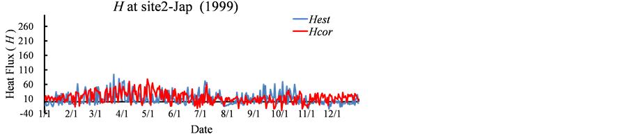


Figure 4. Yearly change of lE and H observed and estimated (W∙m−2) (general solution). Note: Initial condition and constraints are the same with Figure 3.


Figure 5. Comparison of lE and H observed and estimated (W∙m−2). Note: Initial condition and constraints are the same with Figure 3.


Figure 6. Hourly change of rehs and Ts (general solution). Note: Initial condition and constraints are the same with Figure 3.
shows the change of Ts − T0 and Ts − Tz. The Ts changed remarkably from initial value T0. The Ts − T0 changes a difference ranging from −10˚C to +10˚C at site1-Jap and ES-VDA while −3˚C to +2˚C at US-Kon, US-Goo and IE-Dri, and from −3˚C to +12˚C at US-Br2. The difference Ts and Tz is about −10˚C to +12˚C, which has no site specific trends. The above features of rehs and Ts changes are quite similar to the other that in season although they have a small difference.
Seasonal change of the lE and H at the all sites is also investigated. The feature has not remarkable difference among February, May, Jun-July, September and November, although the quantity has season specific changes.
3.6. Slope of Estimated against Observed in All Analyzed Data
Table 5 describes all analyzed daily data at tested six sites including observed and corrected versus estimated using the proposed method for lE and H as well as Ts versus T0 with rehs versus rehz. The feature is site specific. For corrected against estimated lE and H, the relationship is already described by Figure 5.
For lEobs versus lEest, IE-Dri and ES-VPA are overestimated (>15%). For Hobs versus Hest, US-Goo and ES-VPA are overestimated while the other sites are underestimated. (<±15%).
The Ts versus T0 relationship are strongly correlated for all sites. The relationship of rehs versus rehz is also strong randomized at site-Jap and US-Br3, US-Kon remarkably
Table 5. All data analyzed by general method (general solution).
Slope express the gradient of estimation (lEest, Hest) against correction (lEcor, Hcor) and observation (lEobs, Hobs), Initial condition rehs = rehz, b > 0. Note * indicates ±15%. Note: initial cindition at site2-Jap, US-Br3, IE-Dri and ES-VDA are rehs = 1.0. US-Kon and US-Goo are rehs = rehz. Constraints: at site2-Jap, US-Br3, IE-Dri and ES-VDA are b > 0. US-Kon and US-Goo are b < 0.
randomized.
3.7. Comparison of Estimated and Observed Evapotranspiration Rate (ETa)
Using observed and estimated lE, monthly evapotranspiration was obtained at the all sites, as shown in Figure 7 by assuming 100 W∙m−2 equivalents for 3.53 mm∙day−1 [12] . The initial value of rehs and constrains are chosen as aforementioned. If there are data gap in a given month, the monthly average ETa obtained as follows: The average ETa in a day multiplied the number of days of the month.
All sites describe very well reproduced the monthly change of ETa. In detail, although there are small differences between ETaobs, ETacor, and ETaest at all sites, the difference was relatively small.


Figure 7. Comparison of observed (ETaobs) and estimated (ETaest) monthly evapotranspiration (mm∙month−1). Note: Initial condition and constraints are the same with Figure 3. Observed data attached as reference.
Besides the pattern of monthly changes, the total amount of the ETa is summarized in Table 6. The amount of annual lEest and Hest are satisfactorily consistent with lEcor and Hcor or lEobs and Hobs, i.e., ETaest/ETacor (<±15%) excluding US-Kon. US-Kon has big imbalance 140 mm∙year−1 even if after correction by regression analysis. The other sites have a relatively small imbalance. The facts describe that ETa can be estimate by our method within 85% accuracy.
4. Consideration
4.1. Relationship of Penman Method with Proposed Method
To verify the validity of our method, our method was compared with penman method. Penman method is used to evaluate evaporation from the saturated or wet soil surface that corresponding to our proposed method as rehs equals to 100%.
Penman evaporation evaluated by Equation (14) [13]
 . (14)
Here, Δ is the slope of saturated vapor pressure curve (hP∙˚C−1) at Tz, γ is hygroscopic constant (hP∙˚C−1), λ is latent heat flux (MJ∙kg−1), U10 is wind speed at 10 m height (m∙sec−1), another variable already described.
Figure 8 describes the comparison of evaporation estimated by Penman method with our proposed method using daily data of Ishikawa Prefectural Forest Experimental Station (Latitude (+N/−S): 36.4309, Longitude (+E/−W): 136.6424) (2014). The result by our method obtained using Equation (3) that optimized Ts at 100% of rehs reproduced well Penman’s result even though a little scattered. The scattered point may produce with observation quality by related climate elements. Our method does not require the wind speed correction that appeared in the second term of right hand side in Penman Equation (14), which was already pointed out by Urano [13] . In addition, constraint of Rn ? G > lE and H is applied.
Table 6. Total amount of evapotranspiration estimated and observed including correction (mm∙year−1).
Note 1) Initial cindition at site2-Jap, US-Br3, IE-Dri and ES-VDA are rehs = 1.0. US-Kon and US-Goo are rehs = rehz. 2) Constraints: at site2-Jap, US-Br3, IE-Dri and ES-VDA are b > 0. US-Kon and US-Goo are b < 0. 3. Imbalance: (Hest + lEest) − (Hcor + Hobs). Note * indicates ±15%.


Figure 8. Comparison of Penman method with our method (W∙m−2).
4.2. Comparison of Bulk Transfer Method at Wetted Soil Surface with our Method
Furthermore, to obtain more reasonable result, we applied the Bulk Transfer Concept (BTC). The heat balance equation of the BTC can be expressed as Equation (15) [14] . The third term of left hand of the equation expressed the sensible heat flux and the fourth term expressed the latent heat flux. Before optimization, Equation (15) is not closed because CH, CE and Ts are assumed. The optimization conducted as the ε goes to minimum.
 . (15)
Here, CH is bulk transfer coefficient of sensible heat flux, CE is bulk transfer coefficient of latent heat flux, Uz is wind speed, other variables already described.
As described in Figure 8, our method using Equation (15) with the condition of CH = CE, that is the same of Penman method’s assumption [14] , is very well reproduced, although the procedure does not unified the variables CH = CE and Ts mathematically because one equation determine two variables.
4.3. Comparison of Observed Ts with Estimated by Radiometer Ts
To verify the reasonability of estimated Ts, Figure 9 compares the estimated Ts with observed Ts by radiometer at three sites. The sites almost indicate well coincident with each other, thus, the data shows the validity of the Ts estimation.
5. Discussion
5.1. Initial Values and Constraints
There are plural results i.e., local minimum, as satisfying Equation (8) and Equation (9) at different initial values because of nonlinear simultaneous solution. One of the technical points of our research is how to find out the reasonable initial values of Ts and


Figure 9. Comparison of Ts observed by radiometer and estimated (˚C).
rehs with constrains. We approach the final values of rehs and Ts from both sides saturated and observed rehz with constraints of b < 0 or b > 0. The results obtained by this procedure are mostly successful. One important thing is that the initial values Ts and rehs to be set as possible as vicinity to the final values.
5.2. Abnormal Fluctuation of Bapp (Singularity of Bapp)
If Ts approaches zero in convergence process, Bapp is remarkably increased according to approaching zero from the opposite side, positive and negative, as shown in Figure 10. This tendency is almost independent of , although there are small differences. Actually, when denominator of Equation (4) approaches zero
  i.e., rehs approaches to
 , the abnormal Bapp appeared. To avoid this conflict, Bapp is limited to (−100 < Bapp < 100) as aforementioned, referring to the observed and calculated data approximately [1] .
6. Conclusions
In the natural world, the air temperature and humidity reflect the partitioning of sensible and latent heat flux from Rn and G. Based on this concept, we attempt to estimate H

Figure 10. Relationship between Bapp and temperature Ts when Ts − Tz = 1.0˚C [1] .
and lE reciprocally using single height temperature and humidity, and Rn and G by applying the Bowen ratio concept on the soil surface. This feature can be remarkably extended to the field of utilization. The unknown variables Ts and  (i.e., rehs) are estimated by an optimization procedure as satisfying heat balance relationship. The validation of the method was achieved by the six sites in the humid regions of Japan, USA and Europe. lE and H were observed by the eddy covariance method at these sites, except lE in Japan site. Analysis is conducted on an hourly basis and summarized daily. The main results are as follows:
1) The hourly and yearly change of the estimated lE and H very well coincided with the observed values at all sites.
2) The estimated lE and H versus corrected lE and H or observed lE and H are satisfactory coincided.
3) The hourly change of Ts and rehs can be estimated by the method that is very difficult to observe at actual site.
4) The estimated evaporation ETa satisfactorily coincided with corrected and observed ETa not only monthly change but also annual amount.
5) The method compared with penman method and confirmed the validity.
The estimated results have not completely reproduced the observations, but the results are mostly satisfactory. This fact shows that the method is useful for the estimation of lE and H. The remarkable feature of the new method is that it is applicable for the approximate of lE and H using a single height of Tz and rehz with Rn and G. For estimation of ETa, this method will be applicable to various local areas because of required data easily obtained.
But, there are problems that still remain. The error plain i.e., εi in Equation (3) related to Ts and rehs, is very complicated because of nonlinear simultaneous equation having many local minimum. Therefore, the selection of initial values of Ts and rehs is important issue to be solved in future. On the other hand, this research is restricted at humid region but analysis of sensible and latent heat flux at arid and semi-arid region is also very important. This is also another big problem to be solved in future.
We conclude that the partitioning of lE and H is controlled by energy conservation in nature. Realistically, the observed temperature and humidity are strongly affected by the partitioning of H and lE, and vice versa. Therefore, using the observed temperature, humidity and common climate elements, the lE and H values are reciprocally approximated by the optimized techniques.
Acknowledgements
We sincerely thanks for providing the AmeriFlux and EuroFlux principal investigation for data accessed on July 5, 2015. We sincerely thank Dr. Asanuma Jun, a professor at Tsukuba University, for providing valuable data for the eddy covariance method; Dr. Kuwagata Tsuneo, Dr. Fujihara Yoichi and Dr. Takimoto Hiroshi for providing valuable comments on the optimization procedure. We also thank Dr. Yoshida Masashi and Dr. Noto Fumikazu, who are staff members at Ishikawa Prefectural University, for recording the data. We also thank the staff at the Ishikawa Forest Experiment Station.
Cite this paper
Maruyama, T. and Segawa, M. (2016) Application of the Reciprocal Analysis for Sensible and Latent Heat Fluxes with Evapotranspiration at a Humid Region. Open Journal of Modern Hydrology, 6, 230-252. http://dx.doi.org/10.4236/ojmh.2016.64019
References
- 1. Maruyama, T. and Segawa, M. (2016) Reciprocal Analysis of Sensible and Latent Heat Fluxes in a Forest Region Using Single Height Temperature and Humidity Based on the Bowen Ratio Concept. Journal of Water Resource and Protection, 8, 724-742.
http://dx.doi.org/10.4236/jwarp.2016.87059 - 2. Kondo, J. (1996) Meteorology on Water Environment, 6. Water and Heat Balance on Soil Surface. Asakura Publishing Ltd., Tokyo, 128-159.
- 3. Twine, T.E., Kustas, W.P., Norman, J.M., Cook, D.R., Houser, P.R., Meyers, T.P., Prueger, J.H., Staks, P.J. and Wesely, M.L. (2000) Correcting Eddy-Covariance Flux under Estimates over a Grassland. Agricultural and Forest Meteorology, 103, 279-300.
http://dx.doi.org/10.1016/S0168-1923(00)00123-4 - 4. Wison, K., Goldstein, A., Falge, E., Abbinet, M., Baldocchi, D., Berbingier, C., Ceulemans, R., Dolman, H., Field, C., Grelle, A., Ibrom, A., Law, B., Kowalski, A., Meyers, T., Moncrieff, J., Monson, R., Oechel, W., Tenhunen, J., Valentini, R. and Verma, S. (2002) Energy Balance Closure at FLUXNET Sites. Agricultural and Forest Meteorology, 113, 223-243.
- 5. Allen, R. (2008) Quality Assessment of Weather Data and Micrometeorological Flux Impact on Evapotranspiration Calculation. Journal of Agricultural Meteorology, 64, 191-204.
http://dx.doi.org/10.2480/agrmet.64.4.5 - 6. Asanuma, J. (2012) Site2-Jap, Data of Heat and Water Balance Observation, 1999-2011 by CD. Center for Research in Isotope and Environmental Dynamics, Tsukuba University.
- 7. Prueger, J.H. (2010) Brooks Field Site 11 (US-Br3) AmeriFlux L2 Data.
http://cdiac.esd.ornl.gov/programs/ameriflux/data_system/aaBrooks_Field_Site_11_pf.html - 8. Brunsell, N. (2009) Konza Prairie (US-KON) AmeriFlux L2 Data.
http://cdiac.esd.ornl.gov/programs/ameriflux/data_system/aaKonza_Prairie_pf.html - 9. Meyers, T. P. (2006) Goodwin Creek (US-Goo) AmeriFlux L2 Data.
http://cdiac.esd.ornl.gov/programs/ameriflux/data_system/aaGoodwin_Creek_pf.html - 10. Carrara, A. and Gimeno, C. (2008) Vall dAlinya (ES-VDA) European Fluxes Database Cluster L2 Data.
- 11. Kiely, G., Leahy, P. and Foley, N. (2008) Dripsey (IE-Dri) European Fluxes Database Cluster L2 Data.
- 12. Kondo, J. (2015) Heat Balance and Climate on Soil Surface.
- 13. Urano, S.-I. (2012) Study on Bowen ratios in the Penman and Priestly·Taylor Equations. Geophysical Bulletin of Hokkaido University, Sapporo, 15, 91-107
- 14. Kondo, J. (1996b) Meteorology on Water Environment, 5. Wind and Its Turbulence near Soil Surface. Asakura Publishing Ltd., Tokyo, 99-127.
Appendix 1
The GRG Nonlinear Solving Method for nonlinear optimization: developed by Leon Lasdon (University of Texas at Austin) and Alan Waren (Cleveland State University) and enhanced by Frontline Systems, Inc.
For more information about the other solution algorithms, advice on building effective solver models, and solving larger scale problems, contact: Frontline Systems, Inc.
Web site: http://www.solver.com, E-mail: info@solver.com
Estimated results have not completely reproduced the observations, but the results are mostly satisfaction.
Appendix 2
Using modules of Visual Basic for Applications (VBA) in the manuscript
Sub Macro “Number1 ()
' Macro ”Number 1”:GRG method
Dim r As Long
Dim lastRow As Long
lastRow = Range(“〈Column Alphabet〉” & Rows Count).End (xlUp).Row
SolverReset
For r = 〈Start row number〉 To 〈End row number〉
SolverReset
SolverOptions Precision:=0.000001, Convergence:=0.0001, StepThru:=False, Scaling:=False _
, AssumeNonNeg:=False, Derivatives:=2
SolverOk SetCell:= "Row" & r, MaxMinVal:=2, ValueOf:=0_
, ByChange:=Range(Cells(r, 〈First column number〉), Cells(r, 〈Last column number〉))
SolverAdd CellRef:="$ 〈rehs’s Column Alphabet〉" & r, Relation:=1, FormulaText:=1
SolverAdd CellRef:="$ 〈rehs’s Column Alphabet〉" & r, Relation:=3, FormulaText:=0
SolverAdd CellRef:="$ 〈RTs’s Column Alphabet〉" & r, Relation:=1, FormulaText:=5
SolverAdd CellRef:="$ 〈RTs’s Column Alphabet〉" & r, Relation:=3, FormulaText:=-5
SolverAdd CellRef:="$ 〈H estimated’s Column Alphabet〉" & r, Relation:=1, FormulaText:= "$ 〈Rn-G observed’ s Column Alphabet〉$ &r
SolverAdd CellRef:="$ 〈H estimated’s Column Alphabet〉" & r, Relation:=3, FormulaText:=-100
SolverAdd CellRef:="$ 〈LE estimated’s Column Alphabet〉" & r, Relation:=1, FormulaText:= "$ 〈Rn-G observed’ s Column Alphabet〉$ &r
SolverAdd CellRef:="$ 〈LE estimated’s Column Alphabet〉" & r, Relation:=3, FormulaText:=-100
SolverAdd CellRef:="$ 〈Bapp’s Column Alphabet〉" & r, Relation:=1, FormulaText:=100
SolverAdd CellRef:="$ 〈Bapp’s Column Alphabet〉" & r, Relation:=3, FormulaText:=-100
※in case of b>0
SolverAdd CellRef:="$ 〈b estimated’s Column Alphabet〉" & r, Relation:=3, FormulaText:=0
※in case of b<0
SolverAdd CellRef:="$ 〈b estimated’s Column Alphabet〉" & r, Relation:=1, FormulaText:=0
SolverSolve UserFinish:= True, ShowRef:="DummyMacro"
Next
End Sub

Submit or recommend next manuscript to SCIRP and we will provide best service for you:
Accepting pre-submission inquiries through Email, Facebook, LinkedIn, Twitter, etc.
A wide selection of journals (inclusive of 9 subjects, more than 200 journals)
Providing 24-hour high-quality service
User-friendly online submission system
Fair and swift peer-review system
Efficient typesetting and proofreading procedure
Display of the result of downloads and visits, as well as the number of cited articles
Maximum dissemination of your research work
Submit your manuscript at: http://papersubmission.scirp.org/
Or contact ojmh@scirp.org