Journal of Mathematical Finance
Vol.07 No.02(2017), Article ID:76269,11 pages
10.4236/jmf.2017.72016
Application of Fast N-Body Algorithm to Option Pricing under CGMY Model
Takayuki Sakuma
Faculty of Economics, Soka University, Tokyo, Japan

Copyright © 2017 by author and Scientific Research Publishing Inc.
This work is licensed under the Creative Commons Attribution International License (CC BY 4.0).
http://creativecommons.org/licenses/by/4.0/


Received: April 13, 2017; Accepted: May 15, 2017; Published: May 19, 2017
ABSTRACT
The N-body problem is an active research topic in physics for which there are two major algorithms for efficient computation, the fast multipole method and treecode, but these algorithms are not popular in financial engineering. In this article, we apply a fast N-body algorithm called the Cartesian treecode to the computation of the integral operator of integro-partial differential equations to compute option prices under the CGMY model, a generalization of a jump-diffusion model. We present numerical examples to illustrate the accuracy and effectiveness of the method and thereby demonstrate its suitability for application in financial engineering.
Keywords:
Jump-Diffusion Model, CGMY Model, Option Pricing, Cartesian Treecode

1. Introduction
The standard and celebrated model for option pricing in the financial industry has been the Black-Scholes model [1] because of its simplicity. However, it is difficult to capture the realistic behaviors observed in option markets with this model. Recently, jump-diffusion models, which take into account jump behavior of underlying assets, have gained attention in financial engineering (the details are given in [2] , for example). For a European option, researchers have suggested efficient schemes which apply numerical methods such as the fast Fourier transform (FFT) [3] , the Hilbert transform [4] , and the Fourier-cosine (COS) [5] methods. The application of these methods to path-dependent options has also been investigated (for example, [6] ).
One approach to price options under jump-diffusion models is to solve the corresponding partial integro-differential equations (PIDEs) numerically, but the PIDEs include non-local integral operators which make the direct numerical evaluation of PIDEs computationally expensive. An efficient approach for computing the integral term is to use the FFT [7] [8] [9] [10] , but this requires two FFT operations per time-step and direct use of FFT requires either a uniform grid or an additional interpolation scheme [11] . Also, an efficient scheme which transforms the PIDEs to pseudo-differential equations and applies FFT to the equations has been suggested [12] , but this also requires two FFT operations per time-step for path-dependent option pricing.
The present paper introduces an application of the Cartesian treecode [13] which has been used as an efficient algorithm for the N-body problem. The N-body problem, which simulates the interactions between individual particles in a multi-particle system, is an active research topic in physics. However, direct computation for this problem is computationally expensive and there are two major efficient algorithms: the fast multipole method (FMM, [14] [15] [16] [17] ) and treecode [13] [18] . FMM is relatively complicated and the performance is not sufficient for the actual computation. On the other hand, although the com- putational burden of treecode is greater, its implementation is straightforward and easier to use in practice.
Little study has been done on the application of these fast N-body algorithms to financial engineering. One application of FMM called the fast Gauss transform (FGT, [16] ) has been implemented under Merton’s jump-diffusion model [19] to solve the corresponding PIDE [9] . However, its computational efficiency was observed to be poor because the method requires more grid points than the FFT method to achieve similar accuracy. Recently, the improved fast Gauss transform (IFGT, [20] ) has been applied and numerical experiments have shown that this method is more efficient than the FFT method [21] ; however, IFGT can be applied only to Merton’s jump-diffusion models.
In the present paper, we apply another efficient approach, called the Cartesian treecode [13] , to the CGMY model ( [11] [22] ). To our best knowledge, this is the first paper applying treecode to option pricing modeling. Using numerical examples, we examine its computational accuracy and ease of implementation for the computation of the integral operators of the PIDE. The use of the treecode makes the computation of option pricing faster than the original finite difference method without losing accuracy.
Furthermore, we examine whether treecode is also applicable in the field of financial engineering.
2. Cartesian Treecode
In the N-body problem studied in physic, the main goal is to compute the summation of pairwise interactions over the particles in a given system (e.g., gravitational forces of stars in a galaxy or the Coulomb forces of atoms in a molecule). Herein, we consider N particles located at . Then given coefficients and potential which describes some relation between particles at positions x and y, we want to compute
(1)
However, naive computation of the direct summation results in an computational cost. The Cartesian treecode [13] is a type of treecode used to evaluate the screened Coulomb (Yukawa) potential efficiently, which involves potential given by
(2)
The intuitive idea behind treecode is that one imagines wanting to compute gravitational force of a star located at some point . Given clusters of stars which are very far from the target star, instead of summing the gravita- tional force of all the stars in the clusters, if D/r is very small, where D is the size of the cluster and r is the distance of the cluster point from the target point, then we can approximate the force for each cluster as that of a star whose mass is equal to the total sum of the stars in the cluster and is located at the center of the cluster (called the cluster point). Treecode applies the Barnes-Hut algorithm [18] to build a hierarchy of such clusters and employs an efficient recursive compu- tation of (far-field) Taylor coefficients to compute particle-cluster approxima- tions of the screened Coulomb potential, reducing the computational cost from to .
A more concrete explanation of the Cartesian treecode is as follows (see [13] for details). First, particles are divided into a hierarchy of clusters c’s by the Barnes-Hut algorithm,
(3)
Second, truncated expansion of the Taylor series of up to order p around cluster point gives
(4)
For each cluster c, the Taylor expansion is applied if , where r is the
radius of the cluster, R is the distance from to the cluster c, and is the multipole acceptance criterion (MAC) parameter. If the condition is not satisfied, then the children of c are examined, or simple direct summation is applied if the cluster is a leaf of the tree. Finally, substituting (4) into (3) gives
(5)
Because is independent of and is independent of , and can be calculated independently and computation of is more efficient (notice that in order to compute (1), the summation is required at each ). Furthermore, the upshot of this Cartesian treecode is that the Taylor coefficients are evaluated recursively.
Generally, FMM is a more sophisticated model for N-body problems in the sense that it also uses near-field expansions, which reduces the computational cost from to , but the additional use of near-field expansions complicates the algorithm and affects the actual performance, whereas the treecode method is simple and straightforward to implement.
3. Application to Solving a PIDE
We apply the Cartesian treecode to option pricing under the CGMY model with diffusion coefficients ( [11] [22] ). We assume the underlying stock price S to follow a jump process so that the European option price satisfies the following PIDE (see [2] for details of the model and the derivation of the PIDE):
(6)
where r is the risk-free rate, q is the dividend, t is the time to maturity, and is the jump measure. The initial condition is given by
(7)
where K is the strike price. Substituting gives
(8)
with
(9)
The major drawback of this approach is that we need to compute the integral operator given in this PIDE at each time-step; however, use of the Cartesian treecode makes this efficient. Under the CGMY model, is expressed as
(10)
for , , , and . The CGMY model has both finite and infinite activity: in the case of , it has finite activity. Also, the CGMY mo- del has both finite and infinite variance: if , the process has finite variance, whereas it has infinite variance in the case of . As mentioned previously, the CGMY model is a generalization of a jump-diffusion model in the sense that corresponds to what is also referred to as the variance gamma (VG) model [23] and corresponds to Kou’s jump-diffusion model [24] .
Furthermore, a more general jump-diffusion model exists known as the generalized tempered stable model [2] ,
(11)
for and , and application of the Cartesian treecode is straightforward.
For numerical evaluation of the PIDE, we employed a simple scheme of the Crank-Nicholson method for the case of a uniform discretization of points, and , where and represent the numbers of dis- cretization points and time steps, respectively. Under this scheme, we decom- pose the integral part as
(12)
where we employ the following approximation [25] for the last term:
(13)
Then the PIDE is solved numerically via a simple Crank-Nicholson scheme:
(14)
where
The boundary conditions are given by
Use of an iterative scheme [11] is also possible as a means of maintaining second-order accuracy with respect to time, but for simplicity and are computed explicitly. is computed via the Cartesian tree- code and in this case the Taylor coefficients of are computed recursively as described in the next section. In the numerical evaluation of , , and , approximation using the trapezoid rule is employed. In addition, the construction of the hierarchy of clusters is executed only at the initial time-step because the grid points are fixed under the Crank-Nicolson scheme.
4. Recursive Computation of
The Taylor coefficients can be evaluated as follows. Let and where . Then and differ-
entiating with respect to z k times ( ) gives
(15)
On the other hand,
(16)
and differentiation with respect to z k times ( ) gives
(17)
From (15) and (17), we get
and
(18)
Finally, dividing by and substituting and gives the following recursive equation for :
(19)
5. Numerical Examples
1The code is available at https://bitbucket.org/cdcooper/yukawatree
We conducted the following numerical experiments, which were executed in Python. The following parameter settings were used [22] : r = 0.06, q = 0.00, C = 0.42, G = 4.37, M = 191.2, Y = 1.0102, and T = 0.25. In the case of the Cartesian treecode, we used publicly available Python code1 using the settings , P = 15, and MP = 30, where is the maximum number of particles in each node of the hierarchy of clusters, and so using a smaller value for MP results in a deeper hierarchy of clusters. The vertical axis in Figure 1 above indicates the price error computed as the difference between the reference price of the Fourier transform method [3] and the price computed using (14), where is computed using the Cartesian treecode (Treecode 1). Treecode 2 indicates the difference between the reference price of the Fourier transform method [3] and the price whose is computed at only one-eighth the number of grid points equally distributed and spline interpolation is employed for the other grid points. The vertical axis in Figure 1 bellow indicates the computation time in case of Treecode 1 and Treecode 2. As shown, there is little difference in Price Error between the cases of FFT and Treecode 1.
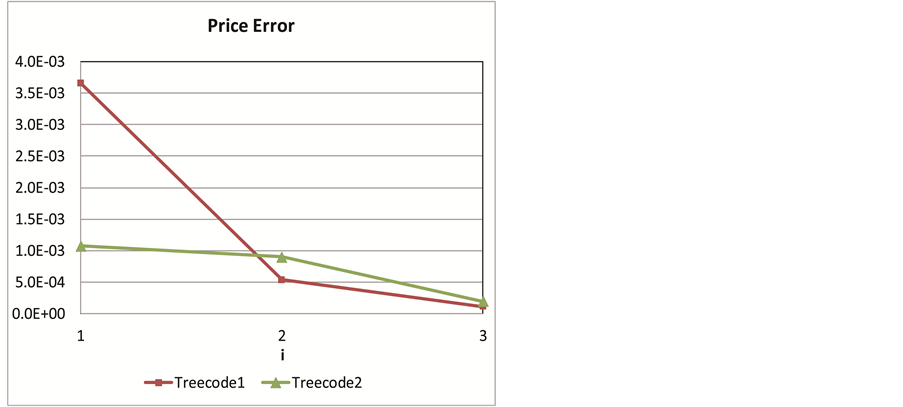
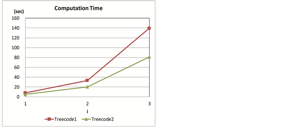
Figure 1. Comparison of price errors and computation time (S = 100, K = 100). The horizontal axis i indicates the integer i used in the numbers of discretization points and time steps under the Crank-Nicolson scheme (14): for .
The flexibility of treecode allows it to achieve higher efficiency of decreasing computational time by choosing target grid points to compute , as is done in Treecode 2.
For Treecode 2, because is a smooth curve with respect to , it suffices to only compute one-eighth the number of grid points equally distributed and interpolating the other grid points via a spline scheme for evaluation of . As shown in Figure 1, we can achieve similar price errors in the case of Treecode 2, while reducing computational time. This method would be especially useful for path-dependent option pricing and a detailed investigation is left for future research.
Figure 2 shows the price and delta values of a European call under the CGMY model for different values of Y using Treecode 2. Here, Y = 0.75 indicates that the process has finite variance and therefore the prices are lower than the case of Y = 1.0102, whose process has infinite variance. Figure 3 shows the price and delta values of a European call under the CGMY model with Y = 0.0 (therefore this model corresponds to a VG model) using Treecode 2, where the following parameter settings [26] were used: r = 0.00, q = 0.0, C = 5.9311, G = 20.2648, M = 39.784, Y = 0.00, and T = 0.5. Both figures demonstrate the smoothness of price and delta with respect to stock price.
6. Conclusion
In this article, we describe applying one of the fast N-body algorithms used in physics, the Cartesian treecode [13] , to the evaluation of the integral operator in a PIDE under the CGMY model. Numerical examples are presented and the results verify the accuracy and efficiency of the treecode method. The recursive computation of coefficients is efficient and by choosing the grid points to be computed and applying interpolation for the other grid points, we can achieve

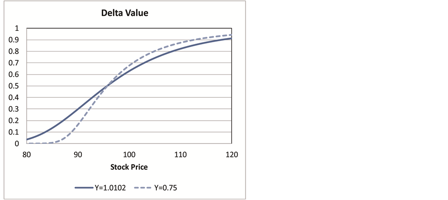
Figure 2. European call option under CGMY model (K = 100): Price and Delta. These are computed using (14), where is computed at only one-eighth the number of grid points equally distributed and spline interpolation is employed for the other grid points.


Figure 3. European call option under VG model (Y = 0.0, K = 100): Price and Delta. These are computed using (14), where is computed at only one-eighth the number of grid points equally distributed and spline interpolation is employed for the other grid points.
high efficiency compared to the original finite difference method without losing accuracy. In addition, the Cartesian treecode can be directly applied to a non- uniform grid, and the use of transformation maps [10] to increase accuracy is also possible. In this paper, we consider a one-dimensional case, but the treecode method is applicable to up to three-dimensional cases, and therefore we can apply the code to a two-dimensional PIDE for pricing basket and spread options. On the other hand, because the treecode method is only applicable to up to three-dimensional cases, the limitation of this approach is that we cannot compute the price of a multi-asset option which involves more than three assets. Application to path-dependent option pricing is also interesting and left for future research.
Acknowledgements
We appreciate Professor Lorena Barba, Simon Layton, and Christopher Cooper for helpful advice and support. I would especially like to note my appreciation of Christopher Cooper for his support in instructing me on how to use his Python code of the Cartesian treecode.
Cite this paper
Sakuma, T. (2017) Application of Fast N-Body Algorithm to Option Pricing under CGMY Model. Journal of Mathematical Finance, 7, 308-318. https://doi.org/10.4236/jmf.2017.72016
References
- 1. Black, F. and Scholes, M. (1973) The Pricing of Options and Corporate Liabilities. The Journal of Political Economy, 81, 637-654. https://doi.org/10.1086/260062
- 2. Cont, R. and Tankov, P. (2004) Financial Modeling with Jump Processes. Chapman and Hall/CRC Financial Mathematics Series.
- 3. Carr, P. and Madan, D. (1999) Option Valuation Using the Fast Fourier Transform. Journal of Computational Finance, 2, 61-73. https://doi.org/10.21314/JCF.1999.043
- 4. Feng, L. and Linetsky, V. (2008) Pricing Discretely Monitored Barrier Options and Default Able Bonds in Jump Process Models: A Fast Hilbert Transform Approach. Mathematical Finance, 18, 337-384. https://doi.org/10.1111/j.1467-9965.2008.00338.x
- 5. Fang, F. and Oosterlee, C.W. (2008) A Novel Pricing Method for European Options Based on Fourier-Cosine Series Expansions. SIAM Journal on Scientific Computing, 31, 826-848. https://doi.org/10.1137/080718061
- 6. Fang, F. and Oosterlee, C.W. (2009) Pricing Early-Exercise and Discrete Barrier Options by Fourier-Cosine Series Expansions. Numerische Mathematik, 114, 27-62. https://doi.org/10.1007/s00211-009-0252-4
- 7. Andersen, L. and Andreasen, J. (2000) Jump Diffusion Process: Volatility Smile Fitting and Numerical Methods for Option Pricing. Review of Derivatives Research, 4, 231-262. https://doi.org/10.1023/A:1011354913068
- 8. d’Halluin, Y., Forsyth, P.A. and Labahn, G. (2004) A Penalty Method for American Options with Jump Diffusion Processes. Numerische Mathematik, 97, 321-352. https://doi.org/10.1007/s00211-003-0511-8
- 9. d’Halluin, Y., Forsyth, P.A. and Verzal, K.R. (2005) Robust Numerical Methods for Contingent Claims under Jump Diffusion Processes. IMA Journal of Numerical Analysis, 25, 87-112. https://doi.org/10.1093/imanum/drh011
- 10. Tavella, D. and Randall, C. (2000) Pricing Financial Instruments: The Finite Difference Method. John Wiley and Sons, New York.
- 11. Wang, I.R., Justin, W.L., Peter, W. and Forsyth, A. (2007) Robust Numerical Valuation of European and American Options under the CGMY Process. Journal of Computational Finance, 10, 31-70. https://doi.org/10.21314/JCF.2007.169
- 12. Jackson, K., Jaimungal, S. and Surkov, V. (2008) Fourier Space Time-Stepping for Option Pricing with Lévy Models. Journal of Computational Finance, 12, 1-29. https://doi.org/10.21314/JCF.2008.178
- 13. Li, P., Johnston, H. and Krasny, R. (2009) A Cartesian Treecode for Screened Coulomb Interactions. Journal of Computational Physics, 228, 3858-3868.
- 14. Boschitsch, A.H., Fenley, M.O. and Olson, W.K. (1999) A Fast Adaptive Multipole Algorithm for Calculating Screened Coulomb (Yukawa) Interactions. Journal of Computational Physics, 151, 214-241. https://doi.org/10.1006/jcph.1998.6176
- 15. Greengard, L.F. and Rokhlin, V. (1987) A Fast Algorithm for Particle Simulations. Journal of Computational Physics, 73, 325-348.
- 16. Greengard, L.F. and Strain, J. (1991) The Fast Gauss Transform. SIAM Journal of Scientific and Statistical Computing, 12, 79-94. https://doi.org/10.1137/0912004
- 17. Greengard, L.F. and Huang, J.F. (2002) A New Version of the Fast Multipole Method for Screened Coulomb Interactions in Three Dimensions. Journal of Computational Physics, 180, 642-658. https://doi.org/10.1006/jcph.2002.7110
- 18. Barnes, J. and Hut, P. (1986) A Hierarchical O (N log N) Force Calculation Algorithm. Nature, 324, 446-449. https://doi.org/10.1038/324446a0
- 19. Merton, R.C. (1976) Option Pricing When Underlying Stock Returns Are Discontinuous. Journal of Financial Economics, 3, 125-144.
- 20. Yang, C. and Gumerov, R. (2003) Improved Fast Gauss Transform. Technical Report CS-TR-4495, University of Maryland, College Park.
- 21. Sakuma, T. and Yamada, Y. (2014) Application of the Improved Fast Gauss Transform to Option Pricing under Jump-Diffusion Processes. Journal of Computational Finance, 18, 31-56. https://doi.org/10.21314/JCF.2014.276
- 22. Carr, P., Geman, H., Madan, D. and Yor, M. (2002) The Fine Structure of Asset Returns: An Empirical Investigation. Journal of Business, 75, 302-332. https://doi.org/10.1086/338705
- 23. Madan, D., Carr, P. and Chang, E. (1998) The Variance Gamma Process and Option Pricing. European Finance Review, 2, 79-105. https://doi.org/10.1023/A:1009703431535
- 24. Kou, S.G. (2002) A Jump-Diffusion Model for Option Pricing. Management Science, 48, 1086-1101. https://doi.org/10.1287/mnsc.48.8.1086.166
- 25. Almendal, A. (2005) Numerical Valuation of American Options under the CGMY Process. In: Schoutens, W., Kyprianou, A. and Wilmott, P., Eds., Exotic Option Pricing and Advanced Levy Models, Wiley, Hoboken.
- 26. Lee, R. (2004) Option Pricing by Transform Methods: Extensions, Unification, and Error Control. Journal of Computational Finance, 7, 51-86. https://doi.org/10.1287/mnsc.48.8.1086.166