ABSTRACT

Given an asset with value, we revisit the Black and Scholes dynamics when the driving noise is a non-Gaussian super-diffusive stochastic process with variance of the type. This super-diffusive quadratic variance behavior, synthesizes a ballistic component which would occur in strongly fluctuating environments. When, the assets can, with high probability, be driven towards the bankruptcy. This extra dynamic feature significantly affects the management of an optimal portfolio. In this context, we focus on basic decisions like: 1) determine the optimal level to sell the asset; 2) determine how to balance a portfolio which incorporates such a high volatility asset; and 3) when facing incertitudes on the asset’s growth rate, construct an optimal adaptive portfolio control. In all mentioned cases and despite the presence of this highly non-Gaussian noise source, we are able to deliver simple exact and fully explicit optimal control rules.

1. Asset Dynamics Driven by a Super-Diffusive Noise Source

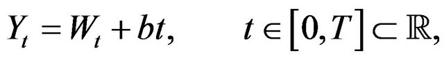
For time, let us consider the basic scalar Black and Schole (BS) type dynamics

(1)

where the driving process is generally a not White Gaussian noise (WGN) stochastic process. In presence of such a general noise source, the solution process Equation (1) is generally not Markovian. Accordingly, besides the initial position, additional information regarding the state of the noise source is mandatory to characterize the time-dpendent statistical properties of. Contrary to the “classical” BS driven by the WGN, optimal asset management, based on optimal stopping rules and/or optimal dynamic portfolio composition, cannot be taken based solely on information of the asset’s value level at a given initial time. This seems truly natural, indeed decisions taken under random environments often rely not only on but possibly on additional features characterizing the underlying fluctuation processes, in particular non vanishing correlations. Hence, often actual applications requires that one escapes the pure WGN’s world. In finance, this aspect has been essentially pioneered in [1] and subsequently it triggered a strong research activity involving non-Gaussian volatility models. Another, though intimately related, dynamic feature of the environment is definitely played by correlations affecting the assets volatility. This last aspect motivated a former work of ours [2], in which we fully and exactly discuss optimal stopping issues for the dynamics Equation (1) when is an alternating Markovian renewal process, (i.e. a continuous time twostates Markov chain). In this particular case, besides, the additional information required to construct optimal decisions is the knowledge of the initial state of the noise source, i.e. one basically needs to know whether initially the noise tendency is to increase or decrease the nominal growth rate. As general noise sources are finitely correlated, contrary to the -correlated WGN, they potentially offer a more realistic stylization of actual environment. This general remark contributes to motivate our present note where we shall unveil a class of elementary correlated noise sources in the BS dynamics for which we are still able to analytically master the mathematical description. In the sequel, for, we focus on the dynamics:

(2)

where the -noise source obeys the scalar diffusion process

(3)

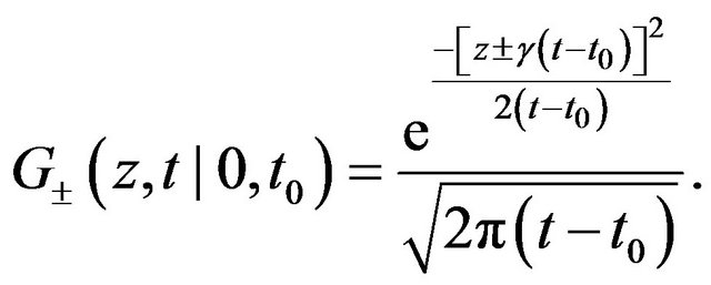
with a given constant and a standard Wiener process. For the highly non-Gaussian process defined by Equation (3), one can nevertheless derive the very simple properties of the transition probability density, (see for examples [3] and [4]):

(4)

with the definition:

(5)

The use of Equation (4) implies that the first moment and the covariance respectively read:

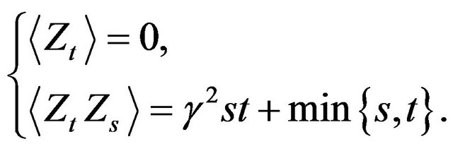(6)

Besides enjoying the simple moments given in Equation (6), it has been shown in [5], that the process is the unique non-Gaussain stochastic process that exhibits Brownian bridges. The superposition of a couple of Gaussian densities appearing in Equation (4), suggests that the process Equation (3) can alternatively be represented in another manner and indeed, as it has been rigorously shown in [6], the realizations coincide with those obtained from the couple of drifted Brownian motions:

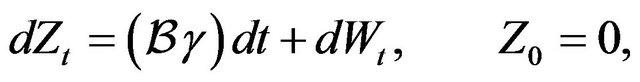(7)

where is a -independent Bernoulli random variable (r.v.) taking the values with symmetric probability. In other words, the process described by Equation (7) should be understood as follows: “at initial time operate the Bernoulli choice of the drift and then evolve according to the resulting -drifted Brownian motion”.

At this stage, we emphasize that the process is a degenerate Markovian diffusion process on the state space. Using the noise representation given by Equation (4) into the basic dynamics Equation (2), we can directly calculate the marginal probability density

and it takes the form:

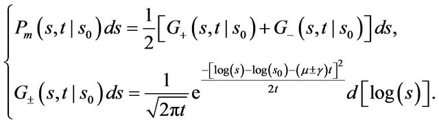
(8)

Hence, for strong ballistic component occurring when, the minus part of the marginal density converges, in the long run, to the Dirac delta probability mass:

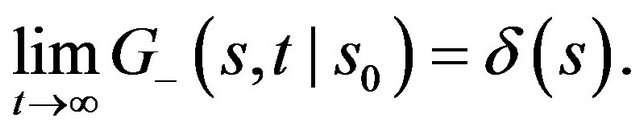(9)

Equation (9) therefore shows that even for strictly positive asset’s growth rate, (i.e.), the superdiffusive noise in Equation (2) can actually drive the process towards the bankrupt state with probability given by Equation (8). The possibility to reach a bankrupt state with high probability should prepare us to derive new optimal management policies for such strongly fluctuating assets. At this stage, it should already be clear that the noise source representation in Equation (4) offers a very simple mathematical approach to discuss several non trivial problems in finance and this will be explicitly explored in the next sections.

2. Optimal Level to Sell an Asset

Consider the standard BS dynamics as given by Equation (2) with, (hence). One naturally asks to determine the critical level at which one should optimally sell the asset when the utility function is:

(10)

In Equation (10) is a discounting rate, which will be chosen such that and is a transaction cost. As it is explicitly discussed in Section 10.2.2 in [7], the exact solution of this optimal stopping problem recommends sale of the asset when its value equals or exceeds the optimal level given by:

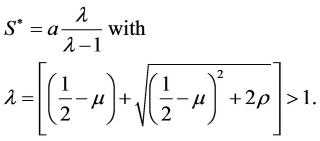(11)

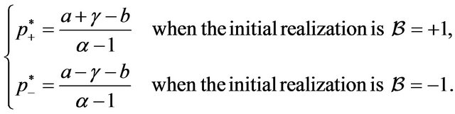
For in Equation (2), the process alone is Markovian. Hence, only the observation of the asset level enables to take the optimal decision. On the contrary, when, the process alone does not remain Markovian, (due to correlations of the noise source), and therefore an optimal selling decision can only be taken if we provide additional information regarding the noise source. The Bernoulli representation in Equation (7) shows that the knowledge of the initial realization of the r.v. is here the required additional information. Once this information is available, one is very directly driven to consider separately the following couple of regimes:

• The realization of the Bernoulli variable is. This implies:

a) never sell the asset (i.e the utility steadily continues to increase leading the stopping time to be).

b) use directly the result given by Equation (11) with the substitution.

• The realization of the Bernoulli variable is. This implies:

a) use directly the result given by Equation (11) with the substitution.

b) bankruptcy is reached with probability and according to Equation (9) one should sell the asset immediately at time.

3. Optimal Portfolio Dynamic Balancing

Here, one asks to determine the optimal portfolio proportion between a risky asset and a fully safe one, in order to ensure that, at a given time horizon, the maximal utility, say, will be achieved. For the WGN driving noise, this problem is explicitly solved in Example 11.2.5 in [7]. The dynamics of the couple of assets reads:

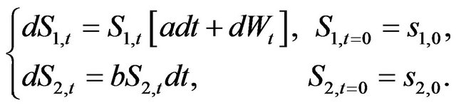(12)

where are the asset’s growth rates. By writing the proportion of the capital invested in the risky asset at time, the resulting capital dynamics evolves as

(13)

For the specific class of utility functions given by:

(14)

it is established in [7] that the optimal proportion is

(15)

Accordingly the optimal portfolio balance will be realized by:

(16)

When replacing in Equation (12) with our correlated noise source defined in Equation (3), the resulting process does not remain Markovian. Hence, the optimal portfolio can only be determined provided additional information on the noise is given. Again this information is contained in the initial value taken by the r.v. in Equation (7). Accordingly, the optimal portfolio composition initially given by Equation (15) now has to be modified to take into account the noise correlations. According to the value taken by, two alternative optimal proportions are found:

(17)

and consequently, the optimal decisions will be given by Equation (16) with the modified proportions given by Equation (17).

4. Adaptive Optimal Control Problem

We have seen in Sections 2 and 3, that, in presence of the ballistic noise source, the construction of optimal decisions necessarily require knowledge of the initial realization of. Now, one may wonder, whether only a partial knowledge of could be compensated by an ad-hoc adaptive control policy enabling, as time evolves, to estimate part of the missing information. Specifically, let us assume that we a priori know the value of in Equation (3) but we however ignore the actual realization initially taken by. As time evolves, an ad-hoc estimator gains sufficient information on to enable the construction of optimal stategies. This problematic has been formalized by I. Karatzas [8] for WGN driving noise. In this section, we will extend Karatzas’ results for the noise source. Following the lines exposed in [8], we start by considering the stochastic process:

(18)

where is a random variable with known probability density. The r.v. is assumed to be independent of the Wiener process. We further assume that neither the process nor the value of can be observed directly. Observations can however be made on the process itself and we define;

(19)

In Equation (19), we introduce a control process which aims at maximizing the probability to reach the right-endpoint of the interval within a fixed time horizon. To fix the ideas, one may for example interpret the process to represent the logarithm of an asset value as in Equation (1). Let us write for the value function of the resulting adaptive optimal control problem (AOCP) and therefore we formally express:

(20)

Writing the corresponding optimal control, Equation (20) therefore reads:

In a remarkable contribution [8], Karrazas solves the above AOCP for pure BM noise sources. For this case, is shown to obey a dynamic programming equation (DPE) exhibiting the form of a parabolic MongeAmpère partial differential equation:

(21)

and Equation (21) is supplemented by a set of appropriate boundary conditions to be found in [8]. The associated optimal control is given by:

(22)

Let us now consider a fully similar problem by replacing the BM with the super-diffusive noise Equation (3). Thanks to the noise representation given in Equation (7), one concludes that when substituting in place of in Equation (18), the Karatzas’ approach and results Equations (18)-(20) can be straight-forwardly used provided one simply modifies the original probability distribution by the convolution:

(23)

Hence, invoking [8] together with Equation (23), two possible regimes differentiated by the support of have to be considered separately:

1) has its support strictly lying on either the positive or the negative axis. In this case, the optimal control policy can be derived and it obeys a certaintyequivalence principle (CEP) holds. To briefly explain the CEP mechanism, assume first that the optimal policy holding when the parameter is known with certainty in Equation (18) is explicitly known. When is unknown but drawn from a probability distribution, the CEP ensures that replacing by a suitable optimal time-depend estimator of yields the optimal control.

2) has its support simultaneously lying on the positive and negative axis. In this situation, [8] shows that drastically different optimal control policy holds.

The previous classification therefore depends intimately on the noise amplitude in Equation (3) and for both situations 1) and 2) and fully explicit results are available, (see Appendix). For large values of, i.e. highly volatile noise sources, (see Equation (6)), the drastic difference between cases 1) and 2) can be traced back to the possibility to effectively have negative drifts (i.e.) with probability. When such negative drifts occur, the use of the certainty-equivalence principle (CEP) is precluded and the resulting optimal control is structurally different.

Explicit illustration. Consider the case where is exactly known and therefore in presence of the noise source. In this case, Equation (23) reduces to

(24)

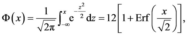
and let us assume that, hence we are in case 1). For the WGN, i.e. when, it follows from the pioneering work [9], (see Appendix), that the corresponding value function and optimal control read:

(25)

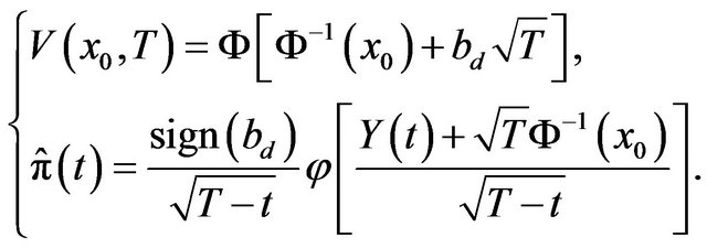
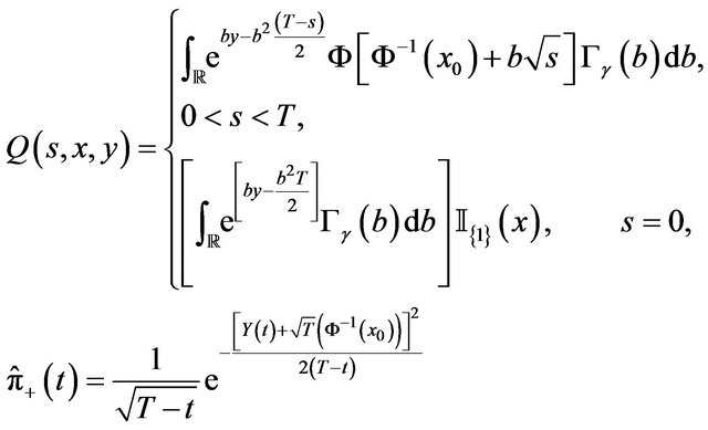
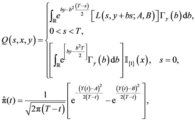
where the notation are given in Appendix, see Equations (29) and (30). Now in presence of the noise Equation (3), i.e. when and assuming, the use of Equation (6.5’) in [8], (i.e. Equation (28) in the Appendix) with Equation (24) implies that Equation (25) has to be modified as:

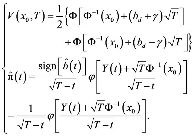(26)

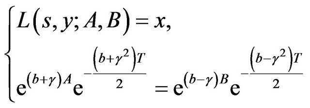
Equation (26) directly follows from the CEP which holds since implies that has a positive definite support. Hence substituting yields the optimal control in presence of the super-diffusive noise. Here the explicit form of the estimator can be explicitly found by using of Equation (4.4) of [8] and Equation (24) and for, we have:

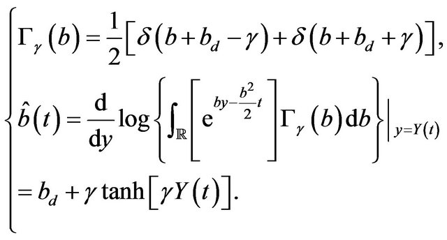(27)

and therefore as already written in Equation (26).

Let us close this section by a couple of remarks:

a) For a given fixed drift, when, and with BM driving noise, the optimal control is given by Equation (25) and its form is independent of the volatility amplitude. This is drastically different for nonGaussian as the volatility amplitude drastically affects the structure of the optimal control;

b) In this model, the information a priori required to construct the optimal control is the volatility amplitude of only and not initial knowledge of the initial realization of. It is the adaptive filtering mechanism which provides the missing information on. This has therefore to be contrasted with the former situations encountered in sections 2 and 3 where both and initial realization of are a priori needed.

5. Conclusion

While several dynamical situations involving stochastic differential equations driven by the super-diffusive noise source Equation (3) have recently received attention in physics [3,4] and various optimal control problems [10], the use of this noise source in finance remains yet unexplored and this motivates our present note. As the super-diffusive noise produces a quadratic increase of the variance, (i.e. volatility) with time, it may lead the assets towards the bankrupt state with high probability. When bankruptcy becomes highly probable, one observes rather drastic modifications in all optimal stopping decisions and portfolio’s compositions. These modifications are easily calculated for the super-diffusive noise source Equation (3). This offers the possibility, in a very simple way, to investigate exactly non-Gaussain and correlation’s effects in assets dynamics. The super-diffusive noise source used here provides a simple and quite efficient didactical tool to escape the ubiquitous Gaussian world in which most exactly soluble models belong.

6. Acknowledgements

This work has been partially supported by the Swiss National Foundation for Scientific Research. I benefit from constructive discussions with Dr. R. Filliger and Dr. F. Hashemi.

REFERENCES

Appendix

Here we simply list, some of the results derived in [8]. For and, we have:

Case 1), Probability distribution has positive support:

(28)

where we use the notation:

(29)

(30)

For the case probability distribution with purely negative support, the situation is, up appropriate signs changes, entirely similar and we do not reproduce it here.

Case 2) Support of the probability distribution without definite sign.

For and and the notation ,:

(31)

where:

(32)

and, for fixed and, the quantities are determined by the couple of transcendent equations

(33)

and the optimal value function reads .

REFERENCES

- O. E. Barndorff-Nielsen and N. Shepard, “Non-Gaussian Ornstein-Uhlenbeck-Based Models and Some of Their Uses in Financial Economics,” Journal of the Royal Statistical Society, Vol. 63, No. 2, 2001, pp. 167-241.
- R. C. Dalang and M.-O. Hongler, “The Right Time to Sell a Stock Whose Price Is Driven by Markovian Noise,” Annals of Applied Probability, Vol. 14, No. 4, 2004, pp. 2176-2201. doi:10.1214/105051604000000747
- M.-O. Hongler, R. Filliger and P. Blanchard, “Soluble Models for a Dynamics Driven by Super-Diffuisve Noise,” Physica A: Statistical Mechanics and Its Applications, Vol. 370, No. 2, 2006, pp. 301-315.
- M.-O. Hongler, R. Filliger, P. Blanchard and J. Rodriguez, “On Stochastic Processes Driven by Ballistic Noise Sources,” In: A. Adhikari, M. R. Adhikari and Y. P. Chaubey, Eds., Contemporary Topics in Mathematics and Statistics with Applications, Asian Books Private Ltd., New Delhi, 2003.
- I. Benjamini and S. Lee, “Conditional Diffusions Which Are Brownian Bridges,” Journal of Theoretical Probability, Vol. 10, No. 3, 1997, pp. 733-736. doi:10.1023/A:1022657828923
- L. C. G. Rogers and J. W. Pitman, “Markov Functions,” Annals of Probability, Vol. 9, No. 4, 1981, pp. 573-582. doi:10.1214/aop/1176994363
- B. Øksendal, “Stochastic Differential Equations—An Introduction with Applications,” Springer, Berlin, 1998.
- I. Karatzas, “Adaptive Control of a Diffusion to a Goal and a Parabolic Monge-Ampère Equation,” The Asian Journal of Mathematics, Vol. 1, No. 2, 1997, pp. 295- 313.
- M. Kulldorff, “Optimal Control of Favorable Games with a Time Limit,” SIAM Journal on Control and Optimization, Vol. 31, No. 1, 1993, pp. 52-69. doi:10.1137/0331005
- R. Filliger and M.-O. Hongler, “Explicit Gittins’ Indices for a Class of Super-Diffusive Processes,” Journal of Applied Probability, Vol. 44, No. 2, 2007, pp. 554-559. doi:10.1239/jap/1183667421