Open Journal of Marine Science
Vol.2 No.2(2012), Article ID:18909,4 pages DOI:10.4236/ojms.2012.22009
Simplified Approximate Expressions for the Boundary Layer Flow in Cylindrical Sections in Plankton Nets and Trawls
SINTEF Fisheries and Aquaculture, Trondheim, Norway
Email: Svein.H.Gjosund@sintef.no
Received January 18, 2012; revised February 24, 2012; accepted March 10, 2012
Keywords: Plankton Nets; Trawls; Non-Tapered Sections; Flow; Boundary Layer; Filtration; Drag
ABSTRACT
Trawls and plankton nets are basically made up of conical and cylindrical net sections. In conical sections the flow will pass through the inclined net wall with a noticeable angle of attack, and then the flow, filtration and drag can be suitably modelled e.g. by a pressure drop approach [1]. In cylindrical and other non-tapered net sections, such as foreparts and extension pieces in trawls and plankton nets, the flow is directed along the net wall and is best considered in terms of a boundary layer. Boundary layer theory and turbulence models can be used to describe such flow, but this requires extensive numerical modelling and computational effort. Simplified approximate formulas providing a qualitative description of the flow with some quantitative accuracy are therefore also useful. This work presents simplified parametric expressions for boundary layer flow in cylindrical net sections, including the boundary layer thickness and growth rate along the net, the filtration velocity out of the net wall, the decrease in mass flux through the net due to the growing boundary layer, and the effect of twine thickness, flow (towing) velocity and the dimensions of the net. These expressions may be useful for assessing the existence and extension of a boundary layer, for appropriate scaling of boundary layer effects in model tests, for proper placement of velocity measurement probes, for assessing the influence on filtration and clogging of plankton net sections, and more.
1. Introduction
When a cylindrical net is towed through water a boundary layer develops and grows in thickness along the inside and outside of the net wall. Mass conservation and pressure boundary conditions imply that a transverse velocity out of the net is induced and that the mass flux through the net decreases downstream. In practice, the boundary layer can be assumed to be turbulent all along the net, and classic turbulent boundary layer results may be used given that the velocity across the wall is small compared to the flow velocity outside the boundary layer, i.e. v/U < 0.01 [2]. Here v is the average normal velocity out of the net wall and U is the undisturbed incident flow (towing) velocity. The porosity, twines and knots of a net constitute a roughness. The classic result for the turbulent boundary layer along a rough wall is the logarithmic law [3], but this is cumbersome to use directly. However, the boundary layer along a rough wall is a modification of that for a smooth wall, for which Prandtl’s simple oneseventh power-law applies. In the following we therefore assume that roughness has a stronger relative influence on the boundary layer thickness than on the shape of the boundary layer velocity profile, and that Prandtl’s powerlaw can be used as an approximation for rough walls also, if the boundary layer thickness is corrected for roughness.
2. Materials and Methods
Prandtl’s one-seventh power-law for the turbulent boundary layer along a smooth plate is given by Equations (1) and (2) [2,3]. Here x is the position along the wall (i.e. the distance from the net mouth), δ(x) is the boundary layer thickness at x, δ(x)/x is the boundary layer growth rate, y is the radial distance from the wall, u(x,y) is the boundary layer velocity profile, U is the undisturbed incident flow (towing) velocity, Rex = Ux/υ and Rex = UL/υ are the relevant Reynolds numbers, υ is the kinematic viscosity, L is the length of the wall, and cf and Cf are the skin-friction and drag coefficients for (one side of) the wall, respectively.
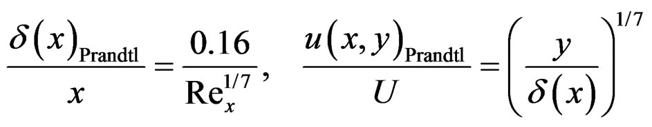 (1)
(1)
 (2)
(2)
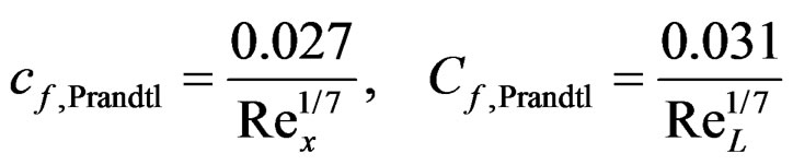
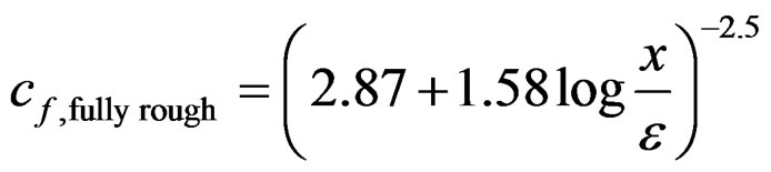
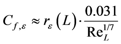
Roughness primarily affects the skin friction coefficient cf, which in turn affects the boundary layer thickness δ(x) and overall drag coefficient Cf. Considering the similarity between Prandtl’s expressions for δ(x)/x, cf and Cf we now assume that a relative increase rε in cf due to a roughness ε results in a corresponding relative increase in δ(x)/x and Cf also, cf. Equation (6). Roughness can be categorized in three regimes; smooth, intermediate and fully rough. Explicit relations for cf exist for the smooth and fully rough regimes, cf. Equations (3) and (4) [2,3], while for the intermediate regime only a complex implicit relation exists (cf. Equation (6)-(82) in [3]). For simplicity we therefore consider all roughness to be in the fully rough regime. This may overestimate the effect of roughness for small and intermediate roughness, but within the scope of the present approach and for the want of a simplified model it seems an acceptable assumption. The ratio rε may now be estimated from Equations (3) and (4). The expression for cf, smooth is only slightly more accurate than cf, Prandtl in Equation (1), but more consistent to use in Equation (5) since cf, Prandtl could result in rε-values less than 1 in some cases. The expression for cf, fully rough applies to so-called sand-grain roughness, which is the most commonly used roughness model.
 (3)
(3)
 (4)
(4)
 (5)
(5)
 (6)
(6)
 (7)
(7)
Figure 1 shows the boundary layer thickness δε(x) estimated from Equation (6) for some values of ε at U = 1 m/s, indicating that the boundary layer growth rate and filtration may be more than doubled for coarse netting compared to very fine netting. Note that while boundary layer thickness generally decreases with increasing velocity, the effect of roughness on the boundary layer thickness increases with increasing velocity, see Figure 2 also. The boundary layer thickness may also be known from observations or measurements, and may then be
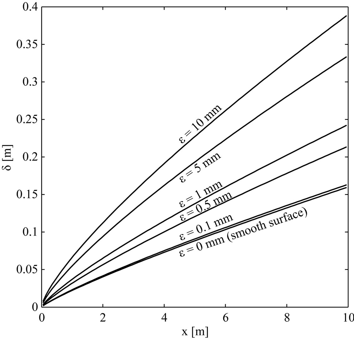
Figure 1. Boundary layer growth along a flat rough wall estimated from Equation (6) for U = 1 m/s and roughness heights ε = 0, 0.1, 0.5, 1, 5 and 10 mm.
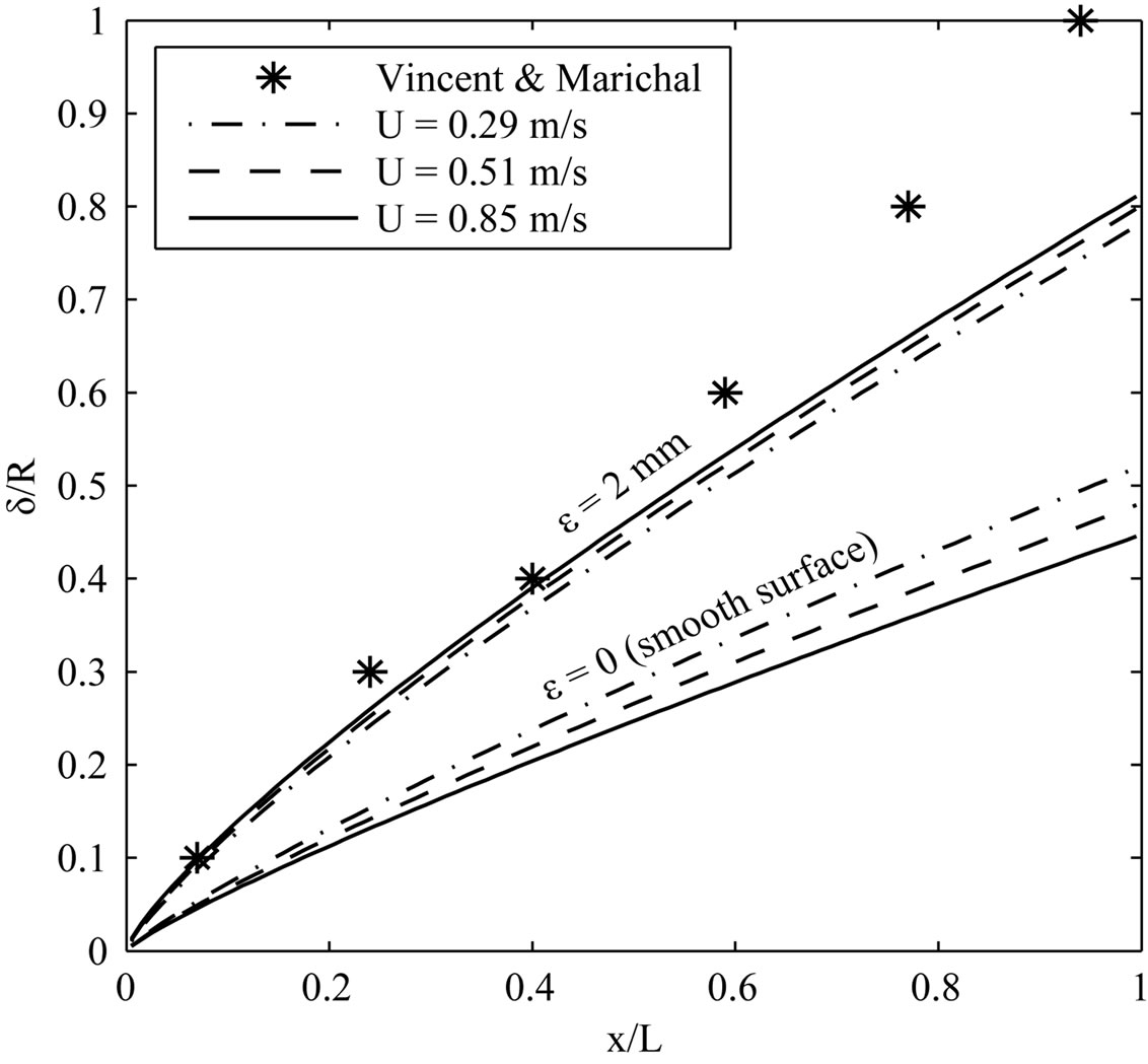
Figure 2. Calculated vs. measured boundary layer thickness for cylindrical net with dtwine = 2 mm, L = 2.2 m, R = 0.1 m for U = 0.29, 0.51 and 0.85 m/s. The measured values for δ/R are approximate values found graphically from the original plots in [4], δ/R for ε = 2 mm are calculated using Equation (6), and δ/R for ε = 0 mm (smooth surface) are calculated using Equation (1).
inserted directly into Equations (8)-(10).
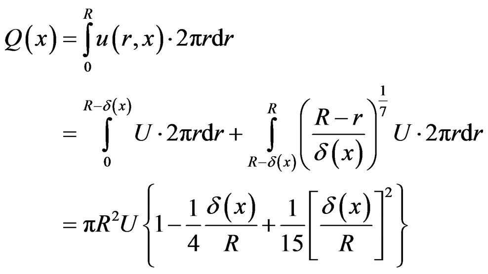
Hence we assume that the boundary layer thickness along a cylindrical net can be approximated by δε(x) in Equation (6), and that the velocity profile across the boundary layer can be approximated by u(x, y)/U = (y/δε(x))1/7. Under these assumptions expressions for the mass flux, radial filtration velocity and drag for a cylindrical net can be found analytically. The mass flux Q through a cross-section of the net is found by integrating the axial velocity over the cross-sectional area, assuming undisturbed flow outside the boundary layer (i.e. in the central core of the net), and using integration by parts for the power law expression, cf. Equation (9). Here R = D/2 is the radius of the net, r is the radial distance from the centreline of the net and y = R – r is the radial distance from the net wall. The radial velocity v(x) across the net wall is found by averaging the loss in Q from x to x + dx over the circumferential strip 2πRdx and making use of Equation (8), yielding Equation (10). The drag coefficient for the cylindrical net, normalized by the frontal area A0, is derived in Equation (11), where L is the length of the net and τw = cf∙ρU2/2 is the wall shear stress. Cf typically lies in the range 0.001 - 0.010 [3]. Note that cf and Cf apply to one side of a wall, and that we must include both the inside and outside of a cylindrical net when calculating the drag.
 (8)
(8)
 (9)
(9)
 (10)
(10)
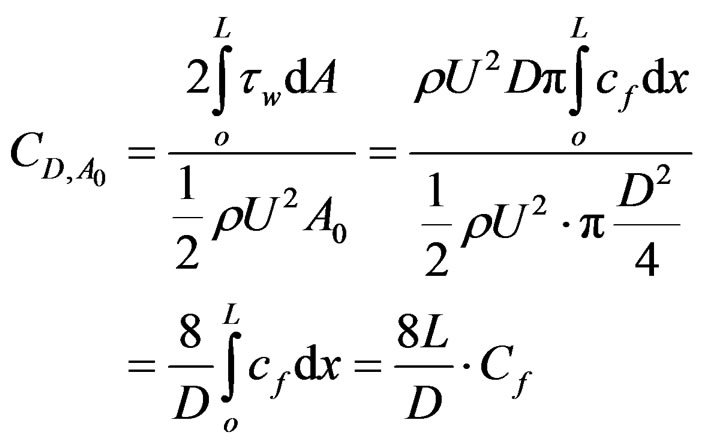 (11)
(11)
3. Results
The simplified expressions in Equations (9)-(11) are compared with experimental measurements from Vincent and Marichal (1996) [4]. They consider an open-ended cylindrical net with L = 2.2 m, D = 0.2 m (L/D = 11), twine diameter d = 2 mm and stretched diamond mesh length lm = 30 mm, for three undisturbed flow (towing) velocities; U = 0.29, 0.51 and 0.85 m/s. There are no noticeable differences between the measured boundary layers for the different velocities in [4], and they are therefore represented by the same markers in Figure 2. The boundary layers calculated from Equation (1) (smooth surface) are clearly thinner than the measured ones, while those calculated using Equation (6) with a roughness height equal to the twine diameter compare quite well with the measurements. The discrepancy is most pronounced towards the open end of the net, which is to be expected since the present simplified model does not account e.g. for end effects or pressure gradients. Figure 2 also shows that when roughness is accounted for the calculated boundary layers for the three velocities nearly merge into a single curve, in agreement with the measurements. Figures 3 and 4 show that the mass flux and filtration velocity are well predicted by Equations (9) and (10), both when δ(x) is corrected for roughness according to Equation (6) and when δ(x) is taken directly from the measurements. Although the boundary layer eventually extends over the entire cross-sectional area of the net, the filtration velocity out of the net wall is small (v ~ 0.01 - 0.001 U) and the filtered volume is modest (less than 20% of the inflow is filtered through the net wall). The drag coefficient can be estimated to CD, A0 ≈ 0.65 for all three velocities (no drag forces or coefficients are given

Figure 3. Calculated vs measured mass flux Q for U = 0.51 m/s.

Figure 4. Calculated vs measured filtration velocity v for U = 0.51 m/s.
in [4]).
4. Discussions
The simplified expressions presented here compare quite well with the measurements in [4]. Comparisons with more measurements are necessary to assess the quantitative performance of the simplified model, but an excellent agreement with accurate measurements cannot be expected. For instance, the present approach neglects the influence of the pressure gradient in the outer region of the boundary layer. This likely explains why the discrepancy with measurements increases towards the open end of the net in Figure 2. Also, since boundary layer theory basically applies to solid surfaces, the present approach is better suited for low porosities than for high porosities, noting that porosity as such is not a parameter in the model.
The present approach may still provide useful estimates of the boundary layer flow in cylindrical net sections in a very simple manner. For fine-meshed netting such as in plankton nets the porosity is low and the roughness small, and then the present approach may be quite representative.
REFERENCES
- S. H. Gjøsund and B. Enerhaug, “Flow through Nets and Trawls of Low Porosity,” Ocean Engineering, Vol. 37, No. 4, 2010, pp. 345-354. doi:10.1016/j.oceaneng.2010.01.003
- H. Schlichting, “Boundary Layer Theory,” 7th Edition, McGraw-Hill, Boston, 1979.
- F. M. White, “Viscous Fluid Flow,” 2nd Edition, McGraw-Hill, Boston, 1991.
- B. Vincent and D. Marichal, “Computation of the Flow Field in the Codend,” Fishing Technology and Fish Behaviour Working Group Meeting, Woods Hole, 5-18 April 1996.