Open Journal of Ecology
Vol.4 No.10(2014), Article ID:48006,9 pages
DOI:10.4236/oje.2014.410052
An Inventory of the Above Ground Biomass in the Mau Forest Ecosystem, Kenya
Mwangi James Kinyanjui1, Petri Latva-Käyrä2, Prasad Sah Bhuwneshwar3, Patrick Kariuki4, Alfred Gichu4, Kepha Wamichwe5
1Department of Resource Surveys and Remote Sensing, Nairobi, Kenya
2Arbonaut Oy Ltd., Helsinki, Finland
3PASCO Corporation, Tokyo, Japan
4Kenya Forest Service, Nairobi, Kenya
5Natural Resource Information & Technology Ltd., Nairobi, Kenya
Email: mwangikinyanjui@gmail.com
Copyright © 2014 by authors and Scientific Research Publishing Inc.
This work is licensed under the Creative Commons Attribution International License (CC BY).
http://creativecommons.org/licenses/by/4.0/


Received 20 May 2014; revised 18 June 2014; accepted 3 July 2014
ABSTRACT
Biomass assessment of the Mau Forest Ecosystem (MFE) was done as part of Kenya’s greenhouse gas inventory. Trans Mara and Mount Londiani forest blocks representing extremes of vegetation types in the MFE were selected for ground data. Based on canopy closure, four forest strata were identified as very dense, moderately dense, open and bamboo. In each stratum, 5 clusters each with 4 plots measuring 30 m × 30 m were located. Big trees (D1.3 ≥ 10 cm) were measured per species for diameter at breast height (D1.3) in the whole plot while height was measured for every 5th tree. Poles (10 cm wang##Bracket# D1.3 ≤ 5) were measured for D1.3 in a 10 × 10 m concentric sub plot. Saplings (5 cm > D1.3; ht ≥ 1.5 m) and seedlings (ht < 1.5 m) were enumerated per species within 5 × 5 m and 2 × 2 m concentric sub plots, respectively. Data were recorded in a Personal Digital Assistant (PDA) and quality checked with Open Foris Collect software. Allometric equations that have been used for similar vegetation in Kenya were used to relate D1.3 and height with biomass. The tree data were uploaded to ArboWebForest (AWF) cloud-service and using the AWF-SIMO calculation tool, average values of diameter, height, and biomass were calculated for each plot. The data were generalised to cover all areas for each block using the Sparse Bayesian linear regression process on the vegetation characteristics with 10 m resolution ALOS-AVNIR-2 images of the MFE. ANOVA was used to compare biomass generated from several allometric equations. Results show that the average biomass of the MFE was 236 Mg·ha−1. Degradation that converts dense forests into open and moderately dense forests contributed to a biomass loss of 228 Mg·ha−1 and 194 Mg·ha−1 respectively. Four allometric equations gave no significant difference (P < 0.05) in biomass for the 80 plots implying that costly processes of developing new equations may not improve accuracy. The study offers a learning lesson in Kenya’s forest inventory processes and the biomass values may show the estimates of stocking in similar forests of Kenya.
Keywords: Forest, Biomass, Inventory

1. Introduction
Through photosynthesis, trees accumulate carbon molecules and store them as a component of biomass [1] . A forest is therefore an accumulation of carbon in plant biomass which has further been classified into pools [2] as above ground representing the trunk, branches, leaves and litter, or below ground comprising the soil and roots [3] . Above ground carbon pools are most prone to changes since they are directly affected by deforestation and forest degradation [4] . For example logging transfers carbon from the forest while fires which burn tree components cause direct releases to the atmosphere [5] . For a forest exposed to various levels of degradation, measuring biomass may show the role of specific disturbance activities on the carbon content of the forest and the specific pools affected [4] .
With less than 20% of Kenya’s land described as high potential [6] , against a growing human population [7] , forests of the country are threatened. In these high potential areas, agriculture and settlement are a priority, and forests have often been excised, totally cleared or over exploited [8] . The Mau Forest Ecosystem (MFE), the most expansive single block of montane forests in Kenya [9] has a long history of degradation. Here, forestland was converted into cropland and settlement [10] ; floristic characteristics of the forest were lost [11] ; biodiversity reduced [12] and vegetation health and density compromised [13] .
The MFE, defined as a montane forest due to its altitudinal placement [14] has two broad forest types [15] . The Afromontane conifer forests found on drier sides of mountains are dominated by indigenous conifers like Juniperus procera (Hochst. ex Endlicher) and Podocarpus latifolius (Thunb. ex Mirb). On the moist sides of mountains, there are the Afromontane mixed forests with broad-leafed species like Polyscias fulva (Hiern. Harms), Prunus africana (Hook. f Kalkman), Macaranga kilimandscharica (Pax) and Tabernaemontana stapfiana (Britten). Reference [11] identified several forest formations that spread among the forest types. These include the Aningeria-Strombosia-Drypetes forest formation with high species richness, occurring at 1600 - 2100 m a. s. l, the Albizia-Neuboutonia-Polyscias formation at 1650 - 2250 m a. s. l, and the Podocarpus latifolius formation with an altitudinal range of 1150 - 2800 m a. s. l. They noted that, these forest formations occasionally overlapped with no clear delineations. There were also areas identified as pure swards of the highland bamboo (Yushania alpina K. Schum). Moreover, [8] observed that Neuboutonia macrocalyx (Pax) and Dombeya torrida (J.F. Gmel) dominated degraded sites in moist and dry forests, respectively.
This study was done with the objective of assembling a set of tools to collect data on above ground biomass which would be incorporated to the remotely sensed data to provide a cost effective method of estimating the above ground biomass content of the MFE and be able to inform a sustainable biomass mapping methodology for the rest of the country.
2. Methods
2.1. Field Plot Sampling
Trans Mara and Mount Londiani Forest Blocks, representing extremes of vegetation types in the MFE were selected for ground data collection. Trans Mara block was quite homogenous, largely comprising of very dense forests of an undisturbed pristine condition. It had characteristics of a moist afromontane forest [15] and represented the vegetation characteristics of the southern blocks of the MFE. Mount Londiani had a variety of vegetation types including bamboo, moderately dense and open forests, showed higher levels of disturbance that opens up the forests, and characterises an afromontane dry conifer forest. The two forest blocks had a total of 51,000 hectares of natural forest.
2.2. Forest Stratification
The forests were stratified using a land-use map based on the categories of the intergovernmental panel on climate change [16] and the category forestland subcategorised to fit conditions of Kenya. Three forest strata were identified on the basis of their canopy closure as very dense, moderately dense and open. In addition, bamboo forest was taken as a fourth stratum due to its unique species composition.
A total of 80 sample plots, distributed into 20 clusters (each having 4 plots) were located among the strata such that each stratum had 5 clusters and 20 plots. Clustering was done to enhance efficiency of measurement, ease of movements and security for the data collection crew. Within a cluster, plots were located 500 meters apart (from plot centre to plot centre) in a square-shaped distribution. There were 64 plots in Mt Londiani block and 16 in Transmara block.
2.3. Field Data Collection
Field work was done between 6th of August and 19th of September 2012. Each sample plot measured 30 × 30 meters in size with three concentric subplots of smaller sizes inside. Big trees, dead or alive (D1.3 ≥ 10 cm) were measured per species for D1.3 in the whole plot while height was measured for every 5th tree in the plot. Poles (10 cm > D1.3 ≤ 5) were measured per species for D1.3 in a 10 × 10 m sub plot, saplings (5 cm > D1.3; ht ≥ 1.5 m) and seedlings (ht < 1.5 m) were enumerated per species within 5 × 5 m and 2 × 2 m concentric sub plots, respectively. Lianas were measured for diameter at 1.3 m distance from the root in the 2 × 2 m concentric sub plot. In the bamboo stratum, culm measurement was done within a 10 × 10 m plot. From each bamboo clump three sample culms for age groups young, mature and old were measured for D1.3 and height.
All D1.3 were measured by diameter tape or calliper while heights were measured with a Trimble Laser Ace rangefinder. Data was recorded using the Open Foris Collect tool [17] into a Personal Digital Assistant (PDA) and the figures recorded to one decimal point. From the PDA, the data was transferred into a laptop and quality checked using the Open Foris Collect while in the field.
2.4. Allometric Equations for Biomass Estimation
Reference [18] reviewed 850 allometric equations for biomass estimation developed for sub Saharan Africa. They categorized the equations as tier 1, 2 or 3. Tier 1 equations had less than 90% accuracy based on probability of expected biomass. Tier 2 equations had more than 90% accuracy but metadata (sample size, range of diameters used and tree components included) was not adequately provided. Tier 3 equations had more than 90% accuracy and had the relevant metadata.
A selection of equations relevant for Kenya was done from [18] . More allometric equations used in Kenya but not available from literature were sampled from relevant institutions. In total 26 allometric equations were interrogated. Using dummy values of D1.3 and height to generate biomass, the 26 allometric equations were ranked according to 1) ability to generate realistic biomass values at all D1.3 sizes, 2) unbiased in residual analysis, and 3) availability of metadata. ANOVA was used to eliminate equations significantly different biomass values. For Lianas and bamboos only single equations were available (Table 1).

Table 1. The ranking of allometric equations used for calculating tree biomass age.
2.5. Analysis of Plot Data
The cleansed data was uploaded to ArboWebForest (AWF) server for further analysis. Averages of D1.3, height and biomass were calculated for trees, saplings, seedlings, lianas, and bamboo in each plot. Height for trees was developed from a height-diameter model (H = 2.4575*D1.30.53155 adjusted R2 = 0.64) generated from data of every 5th tree whose D1.3 and height were measured. For bamboo the equation H = 2.1355*DBH0.8653 (adjusted R2 of 0.48) was used to generate heights of all bamboo culms in a plot.
The allometric equation log10B = (2.18435 × log10(D1.3)) – (0.20922 × log10(D1.3)) – 1.13559 ranked 1st in the review (Table 1) was used to calculate the above ground biomass for trees. For the lianas, the equation B = exp[−1.484 + 2.657lnD1.3] by [21] was used while for saplings and seedlings biomass was calculated based on their numbers as enumerated. For bamboo, biomass per clump was calculated using the only available equation B = 1.04 + 0.06(D1.3*−1.11 + 0.36(D1.3)2) (Table 1). Using the ArboWebForest interface with the AWF-SIMO calculation tool [22] , total biomass from the plant categories (trees, lianas and bamboos) was calculated to give the plot biomass which was converted to per hectare basis using plot size expansion factors.
2.6. Biomass Estimation
Data collected from sample plots was related to satellite image data to provide the overall biomass of the forests. This was done with ALOS (Advanced Land Observation Satellite) AVNIR-2 (Advanced Visible and Near Infrared Radiometer type 2) a 10 m spatial resolution Japanese satellite image [23] . The high resolution allowed capturing of the variety of forest conditions to develop a robust vegetation classification.
With the plot data and satellite imagery as inputs, an estimation model for each forest block was generated using sparse Bayesian linear regression [24] and [25] . A total of 43 Haralick’s textural features [26] were derived from the satellite imagery. These features were calculated separately from image bands; Red and NIR bands of the original image, and the Normalized Difference Vegetation Index (NDVI) image. From each band 13 features were calculated and another four features were calculated as mean values of Green, Red, NIR and NDVI bands.
Correlation reduced the image features from 43 to 22 which were the final input variables for the sparse Bayesian linear regression process. Features that most correlated with the dependent variable, in this case Above Ground Biomass (AGB), and least correlated with each other were used to produce a model which gave the best possible result with least amount of explanatory variables. The model for each block was then used to generate above ground biomass estimates with 30 × 30 m cell size.
2.7. Comparison of Biomass from Various Equations
By generating biomass values differently using each of the 4 best allometric equations (Table 1), ANOVA was used to show the applicability of the other equations in the study area. A test of no significant difference for the 80 plots indicated that either equation would have been used.
3. Results and Discussions
3.1. Biomass Mapping in the MFE
Biomass distribution maps show that Transmara block is homogenous in forest cover and is dominated by the very dense forest stratum. The forest was well stocked recording over 200 Mgha−1 in most areas as indicated by a deep green colours (Figure 1). The lighter green areas with less than 100 Mgha−1 biomass stocking are the bamboo zones while the error class represents the forest area that has been converted to cropland. This biomass map differs from that of Mt Londiani block where biomass varied spatially and gradually reduced from the middle of the forest towards the edges. Here, ground data indicated that very dense forests were only found in inaccessible areas with difficult terrain.
The results show that difference in the conservation status of the two forests with Mt Londiani experiencing a higher level of human encroachment and Transmara forest being relatively well conserved, translates to the biomass content of the forests. The study finds out that the characteristic degradation of forest edges associated with small scale exploitation for subsistence uses documented in several forests of Kenya [8] [10] [12] and [13] compromises the biomass and greenhouse gas sinking processes.
A general map of the MFE showed that the very dense forest stratum was most widely distributed (Figure 2). This is the forest with the highest proportion of biomass. The blocks in the south of the MFE which include Transmara, Maasai Mau and Southwest Mau had expansive areas of very dense forests while those of the north are interspersed with plantations, open forest, moderately dense forests and other land uses. Bamboo forests were found in Transmara, Mt Londiani and Southwestern Mau blocks only. The findings may be used to classify the various blocks of the MFE for the different activities under the REDD+ programme [27] . While blocks in the south of the MFE would be ideal for conservation which retains the existing Carbon, those of the north qualify under enhancement of Carbon stocks through planting programmes.
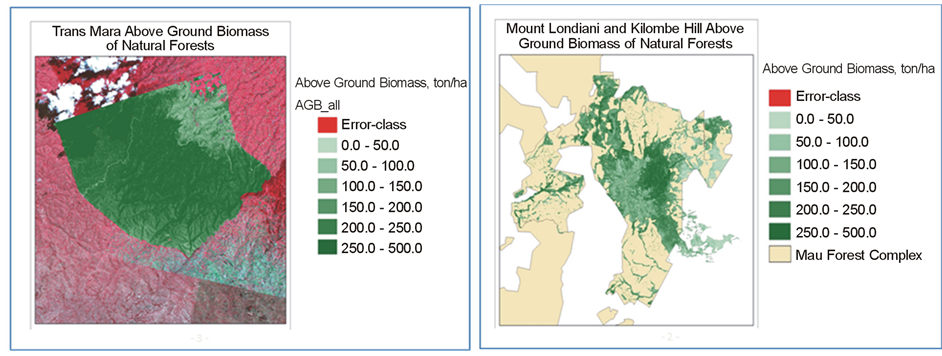
Figure 1. The biomass map for Transmara and Mt Londiani forest blocks.
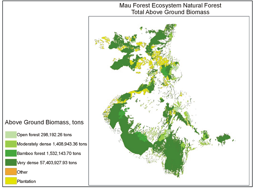
Figure 2. Total above ground biomass map for the MFE.
3.2. Biomass Values in the Selected Blocks
Areas of very dense, moderately dense, open and bamboo forests for the two sampled blocks of forests (Table 2) comprised 82%, 4%, 3% and 12% of the 51,000 ha. The higher extent of very dense forests was attributed to Transmara block where no moderate and open forests occurred. The biomass calculated for the different strata ranged from 265.9 Mgha−1 in very dense forests to 37.78 Mgha−1 in open forests. Transmara block had a better average with 259.74 Mgha−1 as compared to 132.91 Mgha−1 for Mt Londiani. Due to its small area and small average, the open forests constituted an insignificant percentage of the total biomass.
The results imply that deforestation and degradation that converted sections of the dense forest into open forests reduced its potential biomass stocking from 265.9 Mgha−1 to 37.78 Mgha−1, a loss equivalent to 228 Mgha−1. Similarly degradation that gradually opens up a forest reducing its canopy closure may have lost 194 Mgha−1 of biomass, which is the difference between a dense forest and a moderately dense forest. The values show that specific activities of disturbance affect the biomass stocking in the MFE and agree with the findings of [28] who illustrated the effect of encroachment in the volume and yield of the SW block of the Mau forest. The values of biomass loss can be the equivalent potential benefits under REDD+ for forest enhancement in the degraded sections [27] .
3.3. Biomass in the MFE
The average biomass for natural forests of the MFE was 236 Mgha−1. This was influenced by the extent of the very dense forest stratum as compared to the other vegetation strata (Figure 2). The value 236 Mgha−1 is higher than the 190 Mgha−1 default value stated by [29] for moist montane forests. The findings of this study therefore enhance the value of the MFE as a carbon sink beyond the current tier 1 reporting to the UNFCC that uses default values (IPCC, 2013).
The average biomass value of 236 Mgha−1 for the MFE is less than 270 Mgha−1 [9] for the same forest but the two values have no significant difference (P < 0.05). In Kakamega forest in Kenya, [30] reported 249 Mgha−1 carbon biomass for all pools. This would imply about 500 Mgha−1 above ground biomass but the difference can be explained by the difference in conservation status between the two forests which [8] [11] and [13] defined as significantly differing in basal area and other floristic characteristics due to the degradation of the Mau forest and the fact that Kakamega is a tropical rain forest [15] with a higher potential for biomass stocking. Reference [2] obtained a value of 264 Mgha−1 carbon biomass for a tropical forest in the Congo basin and this translates to over 500 Mgha−1 of biomass. This value is associated with the higher biomass content in moist tropical forests of the Congo as compared to Montane forests like the Mau forest.
3.4. Errors of Modeling and Allometric Equations
Models used to estimate biomass in the MFE gave unbiased results with a certainty of 92.8% for the overall forest (Table 3). According to [25] , such accuracy means that the field work was done well. The RMSE values show that the cell values in the biomass maps in Mount Londiani and Transmara forest blocks have on average 77% and 39% of error respectively and these errors are within acceptable levels, when considering that biomass estimation was done using only satellite imagery. The difference between RMSE values between blocks is explained by the difference in vegetation variation. Reference [25] proposes that a plot size bigger than 30 m × 30 m would significantly reduce the error.
There were no significant differences by ANOVA (F0.05(1),3.356 = 0.09475) for the 1st four ranked models (Table 4). As such any of the 4 allometric equations would have been used to calculate forest biomass without major differences in the results. This may imply that the expensive process of developing new allometric equations may not add value to biomass estimation in the study area.
4. Conclusions
This study documents forest inventory methodology used to generate forest biomass data for the MFE. It integrates the use of ground data and high-resolution satellite imagery. This minimises the cost of ground inventory while ensuring accuracy. The study introduces use of technology like the PDA and Open Foris Collect in Kenya where they have not formerly been used and makes data collection and recording easier. Therefore these methods and the recommended improvements like increasing the plot size can be applied to the rest of the forests of
Table 2 . Above ground biomass calculated for the different strata and forest blocks.
Table 3. Modelling errors for the Mount Londiani and Trans Mara models at plot-level.
Table 4. ANOVA table for biomass estimation using 4 different equations.
Kenya to make easy the collection of biomass data which is a requirement for the country’s reporting to UNFCCC regarding greenhouse gases.
A review of allometric equations available for biomass estimation and their application in estimating forest biomass indicates that there are already too many equations in Kenya. Though tree and forest specific equations can enhance the accuracy of biomass estimates, before new equations are developed, the accuracy and applicability of the existing equations should be explored and this would avoid the expensive processes of destructive sampling.
The results of the study enhance the value of the MFE as a carbon. The fact that biomass is higher than the default IPCC value means that the forest has more value than that has been historically estimated. The results indicate the equivalent benefits that would be accrued from enhancement of carbon stocks as well as conservation of the pristine forests and show the specific target areas. This information is necessary for policy makers and would support conservation programmes. It is a justification to conserve the MFE which has been degraded but has many other roles like water catchment and biodiversity.
Acknowledgements
This study was the part of the “Mapping Consultant’s Services”, under the larger project titled “Forest Preservation Programme for the Republic of Kenya”. The project was funded by the government of Japan through Crown Agent’s, Japan. It was implemented by the Kenya Forest Service and PASCO Corporation Tokyo, Japan provided consultant’s services. We appreciate the role of PASCO and Arbonaut in introducing new technology and tools for data collection and analysis.
References
- Sishir G. and Stephan, A.P. (2012) Carbon Pools of an Intact Forest in Gabon. African Journal of Ecology, 50, 414-427. http://dx.doi.org/10.1111/j.1365-2028.2012.01337.x
- Adrien, N.D., Alexander, K. and Gode, G. (2011) Estimations of Total Ecosystem Carbon Pools Distribution and Carbon Biomass Current Annual Increment of a Moist Tropical Forest. Forest Ecology and Management, 261, 1448-1459.http://dx.doi.org/10.1016/j.foreco.2011.01.031
- Fearnside, P.M., Graca, P.M.L., Filho, N.L., Rodrigues, F.J.A. and Robinson, J.M. (1999) Tropical Forest Burning in Brazilian Amazonia: Measurement of Biomass Loading, Burning Efficiency and Charcoal Formation at Alteamira, Pana. Journal of Forest Ecology and Management, 123, 65-79. http://dx.doi.org/10.1016/S0378-1127(99)00016-X
- Losi, C.J., Siccama, T.G., Condit, R. and Morales, J.E. (2003) Analysis of Alternative Methods for Estimating Carbon Stock in Young Tropical Plantations. Journal of Forest Ecology and Management, 184, 355-368. http://dx.doi.org/10.1016/S0378-1127(03)00160-9
- Pastor, J., Aber, J.D. and Melillo, J.M. (1984) Biomass Prediction Using Generalized Allometric Regressions for Some Northeast Tree Species. Journal of Forest Ecology and Management, 7, 265-274.http://dx.doi.org/10.1016/0378-1127(84)90003-3
- Rao, M.N. and Mathuva, M.R. (2000) Legumes for Improving Maize Yields and Income in Semi-Arid Kenya. Agriculture, Ecosystems and Environment, 78, 123-137. http://dx.doi.org/10.1016/S0167-8809(99)00125-5
- Cohen, M.J., Mark, T.B. and Keith, D.S. (2006) Estimating the Environmental Costs of Soil Erosion at Multiple Scales in Kenya Using Energy Synthesis. Agriculture, Ecosystems and Environment, 114, 249-269.http://dx.doi.org/10.1016/j.agee.2005.10.021
- Kinyanjui, J.M. (2009) The Effect of Human Encroachment on Forest Cover, Structure and Composition in the Western Blocks of the Mau Forest Complex. Ph.D. Thesis, Egerton University, Njoro.
- Kinyanjui, J.M., Karachi, M. and Ondimu, K.N. (2012) Documenting the Carbon content of the Mau Forest Complex. Journal of Environment, Natural Resources Management and Society, 1, 70-81.
- Baldyga, T.J., Scott, N.M., Driese, K.N.L. and Gichaba, C.M. (2007) Assessing Land Cover Change in Kenya’s Mau Forest Region Using Remotely Sensed Data. African Journal of Ecology, 46, 46-54.http://dx.doi.org/10.1111/j.1365-2028.2007.00806.x
- Mutangah, J.G., Mwangangi, O.M. and Mwaura, P.K. (1993) Mau Forest Complex Vegetation Survey. KIFCON Report, Nairobi, 134.
- Kinyanjui, J.M., Karachi, M. and Ondimu, K.N. (2013) Natural Regeneration and Ecological Recovery in Mau Forest Complex, Kenya. Open Journal of Ecology, 3, 417-422. http://dx.doi.org/10.4236/oje.2013.36047
- Kinyanjui, J.M. (2011) NDVI Based Vegetation Monitoring in the Mau Forest Complex, Kenya. African Journal of Ecology, 49, 165-174. http://dx.doi.org/10.4236/oje.2013.36047
- Beentje, H.J. (1994) Kenya Trees, Shrubs and Lianas. National Museums of Kenya, Nairobi.
- Prance, G.T. (1984) The Vegetation of Africa. Brittonia, 36, 273.
- Sah, B.P., Hamalainen, J.M., Sah, A.K., Honji, K., Foli, E.G. and Awudi, C. (2012) The Use of Satellite Imagery to Guide Field Plot Sampling Scheme for Biomass Estimation in Ghanaian Forest. ISPRS Annals of the Photogrammetry, Remote Sensing and Spatial Information Sciences, I, 221-226.
- Miceli, G., Pekkarinen, A. and Leppanen, M. (2011) Open ForisInitiave—Tools for Forest Monitoring and Reporting. Concept Note, FAO, Rome, 7.
- Henry, M., Picard, N., Trotta, C., Manlay, R.J., Valentini, R., Bernoux, M. and Saint-André, L. (2011) Estimating Tree Biomass of Sub-Saharan African Forests: A Review of Available Allometric Equations. Silva Fennica, 45, 477-569.http://dx.doi.org/10.14214/sf.38
- Bradley, P.N. (1988) Survey of Woody Biomass on Farms in Western Kenya. Ambio, 17, 40-48.
- Kuyah, S., Dietz, J., Muthuri, C., Jamnadass, R., Mwangi, P., Coe, R. and Neufeldt, H. (2012) Allometric Equations for Estimating Biomass in Agricultural Landscapes: Aboveground Biomass. Agriculture and Ecosystem Environment, 158, 216-224. http://dx.doi.org/10.1016/j.agee.2012.05.011
- Schnitzer, S.A., Mangan, S.A., Dalling, J.W., Baldeck, C.A., Hubbell, S.P., et al. (2012) Liana Abundance, Diversity, and Distribution on Barro Colorado Island, Panama. PLoS ONE, 7, e52114. http://dx.doi.org/10.1371/journal.pone.0052114
- Kangas, A. and Rasinm?ki, J., Eds. (2008) SIMO Adaptable Simulation and Optimization for Forest Management Planning. Department of Forest Resource Management Publications, University of Helsinki, Helsinki, 40.�
- JAXA (2012) Japan Aerospace Exploration Agency. http://www.eorc.jaxa.jp/ALOS/en/index.htm
- Junttila, V., Maltamo, M. and Kauranne, T. (2008) Sparse Bayesian Estimation of Forest Stand Characteristics from Airborne Laser Scanning. Forest Science, 54, 543-552.
- Junttila, V., Kauranne, T. and Leppanen, V. (2010) Estimation of Forest Stand Parameters from Airborne Laser Scanning Using Calibrated Plot Databases. Forest Science, 56, 257-270.
- Haralick, R.M., Shanmugan, K. and Its’hack, D. (1973) Textural Features for Image Classification. Transactions on Systems, Man and Cybernetics, SMC-3, 610-621. http://dx.doi.org/10.1109/TSMC.1973.4309314
- Edwards, D.P., Brendan,F. and Emily, B.(2010) Protecting Degraded Rainforests: Enhancement of Forest Carbon Stocks under REDD+. Conservation Letters, 3, 313-316. http://dx.doi.org/10.1111/j.1755-263X.2010.00143.x
- Kinyanjui, J.M., Karachi, M. and Ondimu, K.N. (2012) Estimating Forest Volume and Yield in the Western Blocks of the Mau Forest Complex, Kenya. Journal of Environment, Natural Resources Management and Society, 1, 59-69.
- IPCC (2006) Guidelines for National Greenhouse Gas Inventories. Volume 4: Agriculture, Forestry and Other Land Use. The Intergovernmental Panel on Climate Change. http://www.ipcc-nggip.iges.or.jp/public/2006gl/pdf/4_Volume4/V4_04_Ch4_Forest_Land
- Glenday, J. (2006) Carbon Storage and Emissions Offset Potential in an East African Tropical Rainforest. Forest Ecology and Management, 235, 72-83. http://dx.doi.org/10.1016/j.foreco.2006.08.014