Open Journal of Ecology
Vol.4 No.4(2014), Article ID:44350,18 pages DOI:10.4236/oje.2014.44020
General Patterns of Spatial Distribution of the Integral Characteristics of Benthic Macrofauna of the Northwestern Pacific and Biological Structure of Ocean
Igor V. Volvenko
Regional Data Center, Pacific Research Fisheries Center (TINRO-Center), Vladivostok, Russia
Email: volvenko@tinro.ru
Copyright © 2014 by author and Scientific Research Publishing Inc.
This work is licensed under the Creative Commons Attribution International License (CC BY).
http://creativecommons.org/licenses/by/4.0/


Received 29 January 2014; revised 28 February 2014; accepted 5 March 2014
ABSTRACT
Horizontal (geographic) and vertical (geonemic) spatial distribution of the integral properties of a large multispecies assemblage (1306 species of fish and invertebrate with body size ≥ 1 cm) from northwest Pacific sea bottom is investigated. There are total number and biomass, average animal size (mean individual weight), species diversity (Shannon’s index) and its components: species richness and evenness (Pielou’s index), i.e. generalized parameters describing benthic macrofauna as a whole. Correlations of these parameters with distance from shore and depth have been found as well as very weak latitudinal zonality display in the region. Even such well-known generalization as Humboldt-Wallace’s law and Bergman’s rule has no noticeable manifestations here. Earlier similar, but not identical, regularities were discovered in the northwest Pacific pelagic water layer. Collation of what there is in the two different sea zones results in new supplements to Zenkevich-Bogorov’s concept of biological structure of the ocean.
Keywords:Benthic Macrofauna; Spatial Distribution; Integral Characteristics; Biological Structure; Northwestern Pacific

1. Introduction
In accordance with the concept of biological symmetry of the oceans by Zenkevich-Bogorov [1] -[4] , the life in the Ocean spreads consistent with 3 symmetry planes (Figure 1). Most stable space regularities correspond to
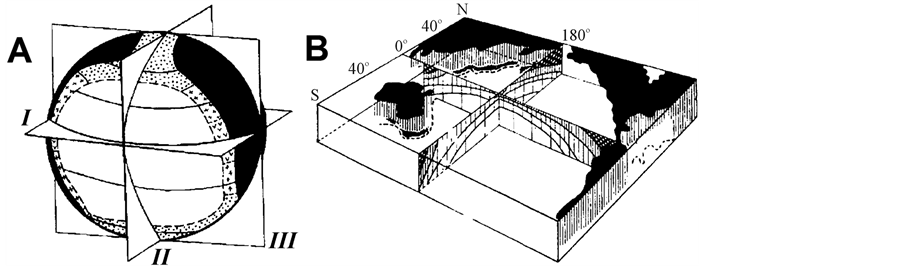
Figure 1. Biological structure of the ocean. At the left (A) symmetry planes are shown: I—equatorial, II and III—meridional (from Ref. [1] ). On the right (B) by shading density the symmetry of Pacific waters productivity is shown (from Ref. [3] ).
three zonality types: latitudinal, circum-continental, and vertical. Primary type of geographic (horizontal) zonality—latitudinal zonality—is conditioned by the spherical shape of the Earth and the unevenness of solar energy incoming on the planet surface. Secondary zonality—circum-continental zonality, which appears in aquatic environment—caused by shallow depths and changed water circulation near the land, it is due to roughness (nonsmooth) surface of our planet.
The most widely recognized latitudinal patterns in ecology and biogeography are: 1) Humboldt-Wallace’s law [5] -[11] —the increase in species richness and/or biodiversity that occurs from the poles to the tropics, often referred to as the latitudinal diversity gradient; and 2) Bergman’s rule [12] -[18] according to which body size of animals increases with latitude. In its pure form, the two patterns on the map of the northwestern Pacific will appear as shown in Figures 2(A) and (B) respectively.
Circum-continental patterns are not so illustrious and have not named someone’s names, but it is for a long time well known that neritic and shelf regions are characterized by higher rates of primary production, biomasses of phytoand zooplankton, benthos, fish and seabirds [3] [4] [19] -[25] . In its pure form, these patterns on the map of Pacific will appear as shown in Figure 1(B), and of the northwestern Pacific—as in Figure 2(D) or Figure 2(E).
A good chance to retest these spatial models appeared a few years ago when, according to the data of 19,436 pelagic trawl stations, carried out by TINRO research vessels in the northwestern Pacific in the waters of an area of nearly 6 mln. km2 (Figure 3) in 1979-2005, general integral characteristics of the macrofauna (which includes 814 species of fish and invertebrate with the body size ≥ 1 cm) have been explored. It was species diversity (H), species richness (S), species evenness (J), total number (N) and overall biomass (M) of all individuals, as well as their average individual weight (W) [26] -[34] . A priori, one would assume that species richness, diversity and average animals weight depicted on northwestern Pacific maps will be distributed in space according to the first (latitudinal) model, and only abundance of animals—to the second (circum-continental).
But it turns out [35] -[37] that integral characteristics of the northwestern Pacific pelagic macrofauna differ in the display of horizontal zonality in the following way: animal’s number and biomass display circum-continental zonality on the regional level (like Figure 2(E)), species evenness and diversity display circum-continental zonality on the global level (Figure 2(D)), animals average individual weight displays two opposite in direction types of circum-continental zonality on the global level (Figures 2(C) and (D))—for various animals and data smoothing levels, species richness doesn’t display any particular zonality (neither latitudinal, nor circum-continental). This list proves different degree of zonality display for different characteristics, and total absence of any latitudinal zonality display in the region (Figures 2(A), (B))—even such famous generalizations as HumboldtWallace’s law and Bergman’s rule are not valid here.
Then, it is assumed [35] -[37] that the absence of the latitudinal zonality display in the region is conditioned by the fact, that meridional (not latitudinal) air and water mass transport prevail here, unlike in southern regions. Collision and interaction between northern and southern, cold and warm waters create a number of local whirlpools, fluid fronts, eddies. This mixed mosaic picture is very changeable in time and space. Apparently, this is exactly what impedes the formation of stable latitudinal gradient of species richness and animal size in this region. This is where Neustruev’s provinciality law [35] [38] proves itself.
It is possible to suppose that in benthal zone (at the bottom and near-bottom layer of water) the action of these
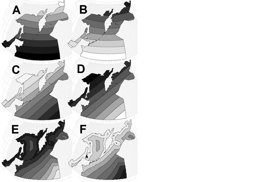
Figure 2. Examples of main geographic patterns: (A) latitudinal zonality on a global level—a parameter decreases from the equator to poles following the solar energy change; (B) invers latitudinal zonality—a parameter increases from the equator to poles; (C) circumcontinental zonality on the global level—a parameter decreases from the center to the periphery of the ocean; (D) the same, but a parameter decreases toward the center of the ocean; (E) and (F) circumcontinental and inverse circumcontinental zonality on a regional scale.
factors is weak, and that is why abiotic environmental factors in animal’s habitat are more stable. This gives the basis to expect that the integral characteristics of benthic macrofauna should be distributed in space of the region in accordance with Humboldt’s law and Bergman’s rule, i.e. latitudinal zoning here is expressed stronger, than circumcontinental.
So whether it is in fact—is a main challenge for present paper.
2. Materials and Methods
The source material for this paper is based on bottom trawl surveys conducted in 1977-2010 by TINRO and its branches for monitoring statuses of ecosystems and biological resources of northwestern Pacific Ocean and adjacent seas (Figure 3). Operate their vessels could only trawl at depths ranging from 5 to 2025 m, so bottom stations are not located at such a great distance from the coast as the pelagic, and cover less area (Table 1). Total in 33 years here was executed 19,151 bottom trawlings that took into account all without exception caught macrofauna, which includes more than 1300 species of fish and invertebrate with the body size ≥ 1 cm (Table 2).
For each station, one-degree trapezoid, water body and for all surveyed area the total abundance of all animals in terms of number N (ind./km2) and biomass M (kg/km2), and also the average individual weight of an individual W = M/N (kg/ind.) have been calculated. As the most widespread measure of species diversity was used the Shannon’s entropic index [39] in interpretation of Margalef [40] :  (bit/ind.), where pi = ni/N is the share of individuals of the i-th species, ni—the number of individuals belonging to the i-th species,
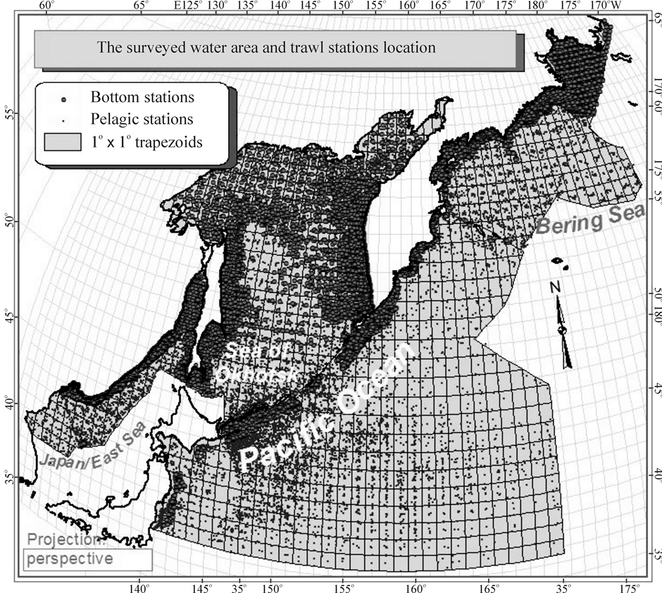
Figure 3. Map of 19,436 pelagic, 19,151 bottom trawl stations, and 955 one-degree trapezia in the surveyed sectors of four water bodies in the northwestern Pacific region with integral characteristics of macrofauna calculated.

Table 1. Sample sizes, on which calculated the integral characteristics of benthic and (in parentheses) pelagic macrofauna.
 —the total number of individuals of all species, S—the number of species or “species richness” (term introduced by McIntosh [41] ). In this way, in ecology H is a measure of uncertainty, unpredictability of the relation of a randomly taken individual to a certain species.
In order to understand biological meaning of a next calculated integral characteristic of biocenotic assemblages, let us first pay attention to the mathematical sense of extremal values of H. Its domain lies in the limits
Table 2. Composition of the studied fauna (number of species).
Note: during a bottom trawling, all these organisms are caught in a trawl with a fine mesh (10 - 12 mm) inserted in its end.
from 0 to  inclusive. At that the H value depends not only on S but also on the relationship of the pi values. The diversity is minimal (H = 0) if one of the pi = 1, all the rest are consequently zero and S = 1. The maximal H value at S > 1 is reached when all probabilities pi are equal, i.e. p1 = p2 = … = pS = 1/S. It is just for this reason that H ≤
 . In ecology, the ratio of real diversity to that maximally possible at the given number of species,
  is called the Pielou’s index [42] . This is an index of uniformity in abundances (equitability), evenness of species in the number of individuals, or sample homoheterogeneity. Its magnitude varies from 0 at S = 1 to 1 at
 . The less J value is, the greater numerical prevalence of few dominant species over all others is.
There are 6 main (or at least those that are most convenient to measure) integral characteristics N, M, W, S, J and H which distribution in space is considered in this paper.
It can be seen on the map (Figure 3) that the surveyed water area does not include the entire Sea of Okhotsk, but the western part of the Bering Sea, the northwest part of the of Japan/East Sea, and a small area of the northwest part of the Pacific Ocean only. Nevertheless, these parts will be called: Japan/East Sea, Sea of Okhotsk, Bering Sea, Ocean, for brevity.
3. Results
3.1. Horizontal Distribution in Basins Scale (Area of 333 - 1368 Thousands km2)
It would be correct to start the large-scale analysis with comparison of the biogeographic zones. However, we need the comparable data regarding the entire Japan/East Sea, as well as the East China Sea and the South China Sea to make it. Non-availability of those data makes us to confine ourselves to comparison of the surveyed areas of three seas, as it was done earlier for macrofauna of the pelagial of the north-west of the Pacific Ocean [34] .
At first, we would like to note that the benthonic macrofauna differs from the pelagic one by higher values of M, W and S. The comparison of the bottom with the pelagial with regard to other characteristics of macrofauna gives mixed results—different for different bodies of water (Table 3). Now let us compare the integral characteristics of the benthal of the Far East seas with each other.
The only characteristic of the benthic macrofauna, for which some regularity is observed, is M. It is gradually increasing from the Japan/East Sea to the Sea of Okhotsk and further on, to the Bering Sea, i.e. from the south to the north (Table 3). Regarding other indices, the “correct” (expected) trend is broken in the Sea of Okhotsk. Thus, for example, W in the Bering Sea is higher than in the Japan/East Sea, but in the Sea of Okhotsk it is lower than in the Japan/East Sea; S and H in the Japan/East Sea are higher than in the Bering Sea, but S value in the Sea of Okhotsk is the highest, and H—is the lowest.
Perhaps, it can be attributed to the significant overlap of latitude ranges, within which these three bodies of water are situated. At this, comparison of such large water areas appears to be too rough.
3.2. Horizontal Distribution in One-Degree Trapezoids Scale (Area of 80 - 9891 km2)
If we consider the spatial distribution of the integral characteristics in more detail—along one-degree trapezoids
Table 3. Integral characteristics of benthic and (in parentheses) pelagic macrofauna of surveyed waters.
Note: characteristics of pelagic macrofauna are taken from [34] .
on the maps (Figure 4), then no apparent latitudinal trend regarding any integral index is observed. It seems that most of them tend to circum-continental distribution within these waters.
Any similarity of actual spatial distributions of any indices to the ideal models discussed in the Introduction can be assessed not only visually on the maps, but quantitatively using elementary statistics. The latitudinal pattern should be characterized by a significant positive or negative correlation between an index examined and geographic latitude, and for circum-continental pattern—between an index and a distance to the shore.
Such analysis shows (Figure 5) that the abundance of the macrofauna tends to increasing in the direction from the south to the north, and the other indices—to decreasing. Yet, for S and H it was to be expected in accordance with the Humboldt-Wallace’s law. However, all and every trends are extremely weak; therefore, they are visually indistinguishable on the maps. N, for which determination coefficient r2 (i.e., proportion of dispersion N, explained by latitudinal gradients) is below 1.7%, is correlated with the latitude more than all other characteristics. For all other characteristics, this value is no significantly differing from zero. It means that the latitudinal zonality in distribution of the integral characteristics of the benthic macrofauna of the surveyed region does not occur practically.
However, the presence of circum-continental trends of all integral characteristics in question is statistically valid here (Figure 6). It was possible to explain only 0.4% - 1.6% of variability of various integral characteristics by latitudinal trend and 1.7% - 14.7%—by circum-continental one. N, M and S decrease, and W, J and H—on the contrary, increase with increasing distance from the shore.
The trends found for the first three characteristics correspond to what is shown in Figure 2(E), and for the next three—in Figure 2(F). The form of relation between the distance to land and S (Figure 6) is worth mentioning. It resembles a right-angled triangle filled with points. This indicates that S variations are maximal near the shore (here it may be few and very many species). With the distance from the land the variance of possible S values is limited by the upper limit, i.e. at a significant distance from the land the number of species can be as little as near the land, but just as many—cannot.
3.3. Horizontal Distribution in Trawl Stations Scale (Area of 0.003 - 1.233 km2)
Within the last of the available spatial scales of integrated data, the latitudinal zonality on the graphs (Figure 7) is also not noticeable. Very weak linear trends are identified here only by regression analysis. At low values of correlation the values of p < 0.01 are only because of the huge number of points.
It is noteworthy that when changing to this scale from the scale of one-degree trapezoids, M maintains a positive and H, S and J—a negative correlation with geographic latitude. However, N changes the correlation from positive to negative one and W—from negative to positive. Based on this, the correlation of the last two variables with the latitude is accidental at all.
The circum-continental trends in the scale of trawl stations (Figure 8) for N, M, W and S retain their orientation and for J and H - changes it from positive to negative. The graphs of these two characteristics in both scale levels (Figures 6, 9) are similar to rectangles filled with points so that for any distance from the shore any values of J and H are found almost equal frequently—from minimum to maximum. This indicates considerable uncertainty of the trends across the entire range of distances from the shore to the point of evaluation of J and H.
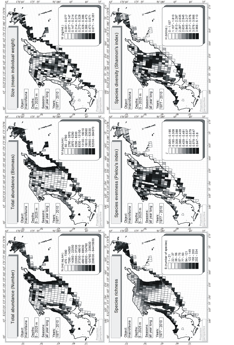
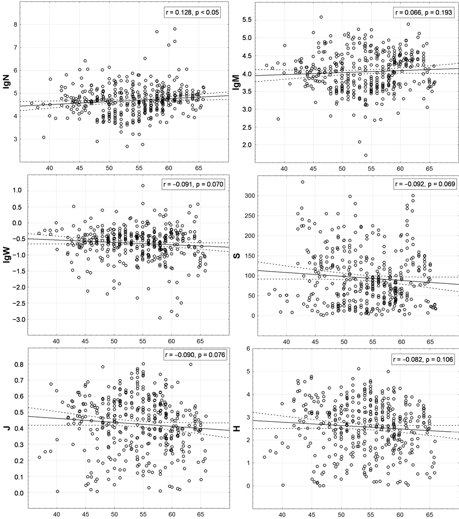
Figure 5. Latitudinal distribution of one-degree trapezoids macrofauna integral characteristics. On axes of abscissa—degree of northern latitude. Here and in the following figures values of Pearson correlation coefficient (r) and p-value for check a significance of its difference from zero are given. The number of points is equal to the number of non-empty one-degree trapezoids on Figure 4.
The distribution graphs of other integral characteristics resemble triangles filled with points (this feature, being faintly visible in Figure 6, appears clearly in Figure 8): isosceles triangles for N, M, W, and rectangular ones—for S. Their shapes indicate that variations of these characteristics are maximum close to the shores—here they can be little and big. With the distance from the land, the variance of possible S values is limited mainly by the upper limit and with regard to N, M, and W on both sides– by the upper and the lower limits.
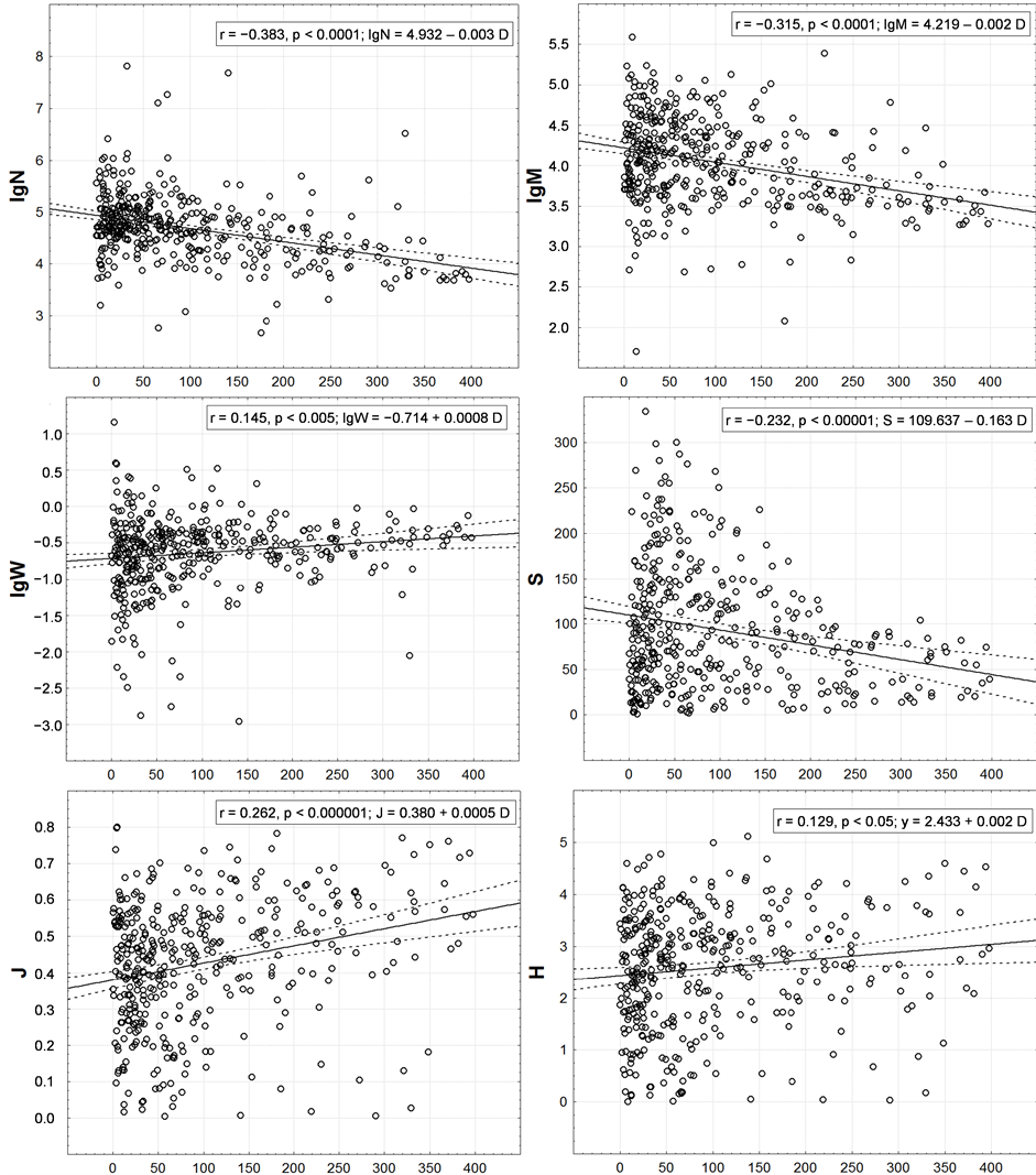
Figure 6. Correlation of one-degree trapezoids macrofauna integral characteristics with remoteness from a coast. On axes of abscissa—distance (km) to the nearest coastline from a centroid of a one-degree trapeze. Except r and p the equations of linear trends are given.
3.4. Vertical Distribution
Now, let us consider the vertical variation of the integral characteristics, i.e. their dependence on the macrofauna habitation depth. Distance to the shore and the same to the water surface (depth) are completely different spatial factors. At first glance, it seems that they should be positively correlated between each other. However, it is not really true in the surveyed region. In the Bering Sea and especially in the Sea of Okhotsk with its extensive shelf, relatively shallow depths are very far from the land, and in the Japan/East Sea and in the ocean near the Kuril
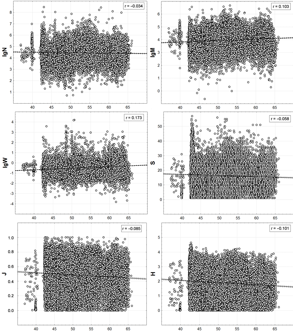
Figure 7. Latitudinal distribution of trawl station macrofauna integral characteristics. On axes of abscissa—degree of northern latitude. Here and in the next figure the number of points is equal to the number of bottom stations shown on Figure 3.
Islands, deep water begins much closer to the shore because of the sharp slope of the bottom. Thus, different depths can occur at the same distance from the shore, and equal depths can occur at completely different distances (Figure 9).
Nonetheless, almost all trends in changing the integral characteristics with changing the depth (Figure 10) are similar to their changes with the distance from the land (Figure 8). The only exception is J: with increase in depth its value increases and decreases with increasing distance. For the reason given in the previous section, it is not surprising.
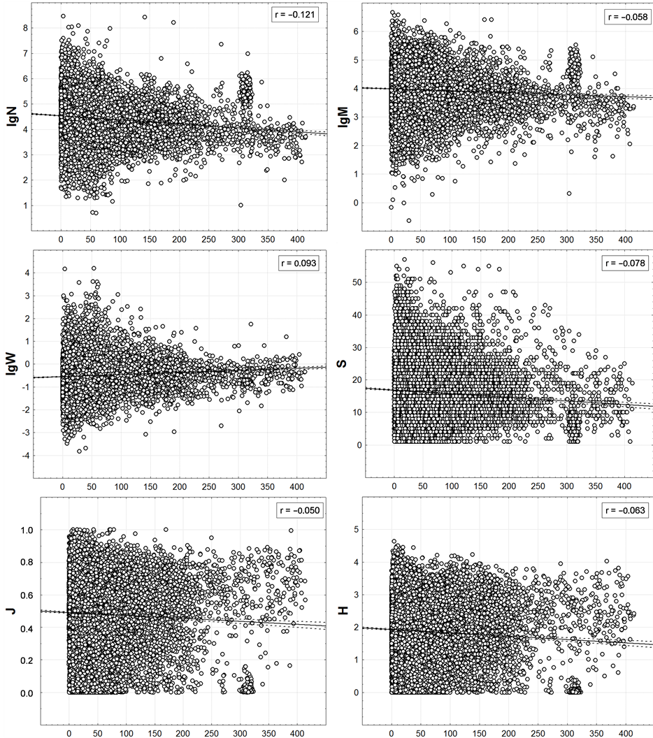
Figure 8. Correlation of trawl station macrofauna integrated characteristics with remoteness from a coast. On axes of abscissa—distance (km) to the nearest coastline from a trawl station position.
The r values indicate that N, M, W and S values depend on the depth more than on the distance to shore. However, based upon the regression coefficients of the linear trends (the second coefficient is equal to the slope ratio of the regression line) 0.00003 - 0.0053 and the determination coefficients of 0.1% - 5.5%, all the correlations shown in Figure 10 are quite weak. They are visually indistinguishable in the graphs, though they are significant (p < 0.01) due to the large number of trawl stations. The clear basic trend, seen by “naked eye”, consists not in it, but in reduction of the variance of N, M, W and S with increasing depth. The same, but to a much lesser extent, is peculiar to J and H.

Figure 9. Correlation of the depths (ordinate axis, m) with distance to a shore (abscissa axis, km) in the centers of one-degree trapezes (at the left) and in sampling points (on the right).
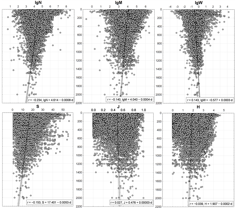
Figure 10. Vertical distribution of benthic macrofauna integral characteristics. On axes of ordinates—depth (m).
Points corresponding to the pelagic trawl stations in this region [35] -[37] , are situated within the same area as the points in Figure 10. They also demonstrate a tendency to reduce the variance of N, M, W with increasing depth, but the linear trends of S, J, and H show reduction in pelagial with decreasing depth and near the bottom they increase for S and H.
4. Discussion
Action of the law of geographical provincialism, which was mentioned in the Introduction, appears in the fact that the areas, biota and communities that are formed historically, mainly under the influence of local azonal factors, become differential within the latitudinal zones. In particular, the topography and geology of the Earth are not subject to zonality. The Russian scientist Neustruyev was among the first to emphasize the importance of local climatic features arising from the specific geographical location and relief of the territory: under their influence, specific interactions of all components, which differ significantly from the zonal ones, arise. Therefore, the law of provincialism or azonality is associated with his family name [38] .
Two regional features of the northwest Pacific are mentioned above:
1) The prevalence of meridional transfer of air and water masses over the latitudinal component of this process2) Small-scale patchiness in the spatial distribution of local whirlpools, fluid fronts, eddies, which prevent the formation of stable latitudinal zonality in the pelagial. Obviously, the influence of these two spatial factors—both, regional and local,—is weakened near the bottom, but there are their analogues having their nuances:
a) Let us note that here the majority of sea bed contours is oriented in the meridian direction (Figure 11(A)). Consequently, the upwelling zones, zones of the coastal convergence of waters, their stratification by the temperature and density, and other characteristics of the benthic habitats are elongated in the same direction. The mature bottom dwellers can expand predominantly in the meridian direction, without leaving their available depth ranges; the drift of their pelagic eggs and larvae from the spawning grounds can be in the same direction.
b) In benthic, the factor of origin plays much more important role compared with the pelagial, including the presence or absence of speciation places in specific areas, share and rank of endemism, as well as the degree of isolation. There is larger habitat diversity at the bottom, and, moreover, benthic inhabitants have more obstacles restricting their expansion compared with the pelagic ones. Besides the physical and chemical properties of the water masses it is the trophic conditions at the bottom and near the bottom, due to the relief features and bottom sediments [43] [44] . Therefore, a variety of community habitats and patchiness in benthic habitat conditions (Figures 11(B), (C)) is even more than in the pelagic zone. In addition, zonality of the bottom by soils and trophic zones largely do not match which increases further patchiness of the benthic community habitats.
However, generalizing the obtained results (Table 4), we can already state that it was possible to find the traces of latitudinal zonality in the benthic. It is expressed very weakly, visually indistinguishable on the maps and graphs, and it is identifiable only by statistical methods (and not always significant). The latitudinal trend appears to the greatest extent in the distribution of M—the biomass of macrofauna increases from the south to the north at all considered scales. Probably, this is due to an increase in the shelf area in a northerly direction in the surveyed waters. As is well-known indeed, the biomass of benthos and nektobenthos on the shelf is more than in the bathyal [44] .
The diversity of H and its components, S and J, decrease to significantly lesser extent in the northerly direction. This trend is so weak that barely identified statistically and it is significant not at all scale levels of generalizing the data. And yet it exists, although it could be not identified at all, as it was during the study of pelagic macrofauna [35] -[37] and demersal fish fauna [45] of the northwest Pacific, or even it could appear to be converse, because we know many cases [46] -[49] when the species richness and/or diversity increases from the equator to the poles, i.e. in the opposite direction to that required by the Humboldt-Wallace’s law.
Theoretically, the Bergman’s rule also does not have to act on the material considered here, as originally it was formulated for warm-blooded animals (see e.g. [18] ), but even for them it is not always valid: regarding the birds it is confirmed only in 71% of cases, regarding mammals—in 65% [50] -[52] . For poikilothermic animals, generally, reverse latitudinal regularity that is often attributed to reduction of the growing season in its length and weight as far as the climate becomes colder is common [53] -[57] . In nature, most exceptions are those cases where the Bergman’s rule is valid for cold-blooded animals. However, on the scale of trawl stations it was found a small but significant positive correlation of the size (mass) of bottom animals with latitude, as it is required by the Bergman’s rule. But it cannot be identified on other scales.
The circum-continental zonality appears on the surveyed water areas much more clearly and independently from the spatial scale of smoothing of data. It is almost identical to the vertical zonality, and it is mainly deter-
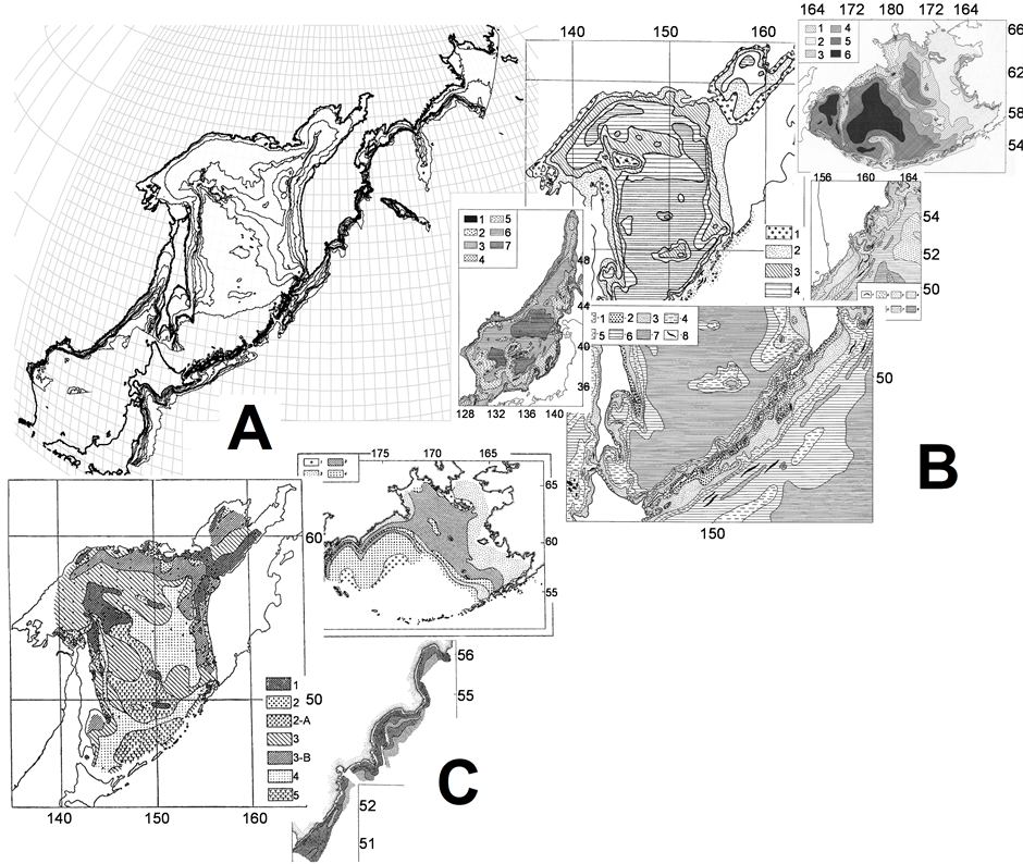
Figure 11. Isobaths (A), bottom sediments (B), and trophic zones (C) allocation in the surveyed region—an illustration from various papers and books Ref. [44]
Table 4. Signs of the integral characteristics mean (m) and variance (v) spatial correlations.
Notes: “+”—increase, “–”—decrease, “0”—without changes, “ ”—no data. Shaded cells indicate statistically significant trends and (for the variance) well noticeable on plots.
mined by it. In accordance with this, the population density N, M and the species richness S decrease with distance from the land and with increasing depth, and the average size of individuals W increases. Also, with distance from shore and with increasing depth the variations of all these characteristics are being reduced significantly. Only J and H are correlated with these spatial factors uniquely.
It should be noted that in this work the effect of circum-continental zonality is detected only at the regional level (Figures 2(E) and (F)). Global trends (Figure 2(C) or Figure 2(D)) for benthal cannot be identified based on the available data due to lack of bottom trawl stations away in the ocean, at depths exceeding 2025 m; the lower right part of the map (Figures 3, 4) is blank. However, through the example of biomass it can be seen that the mapping of the initial data (Figure 12(A)), their averaging (Figure 12(B)) or interpolation (Figure 12(C)) give
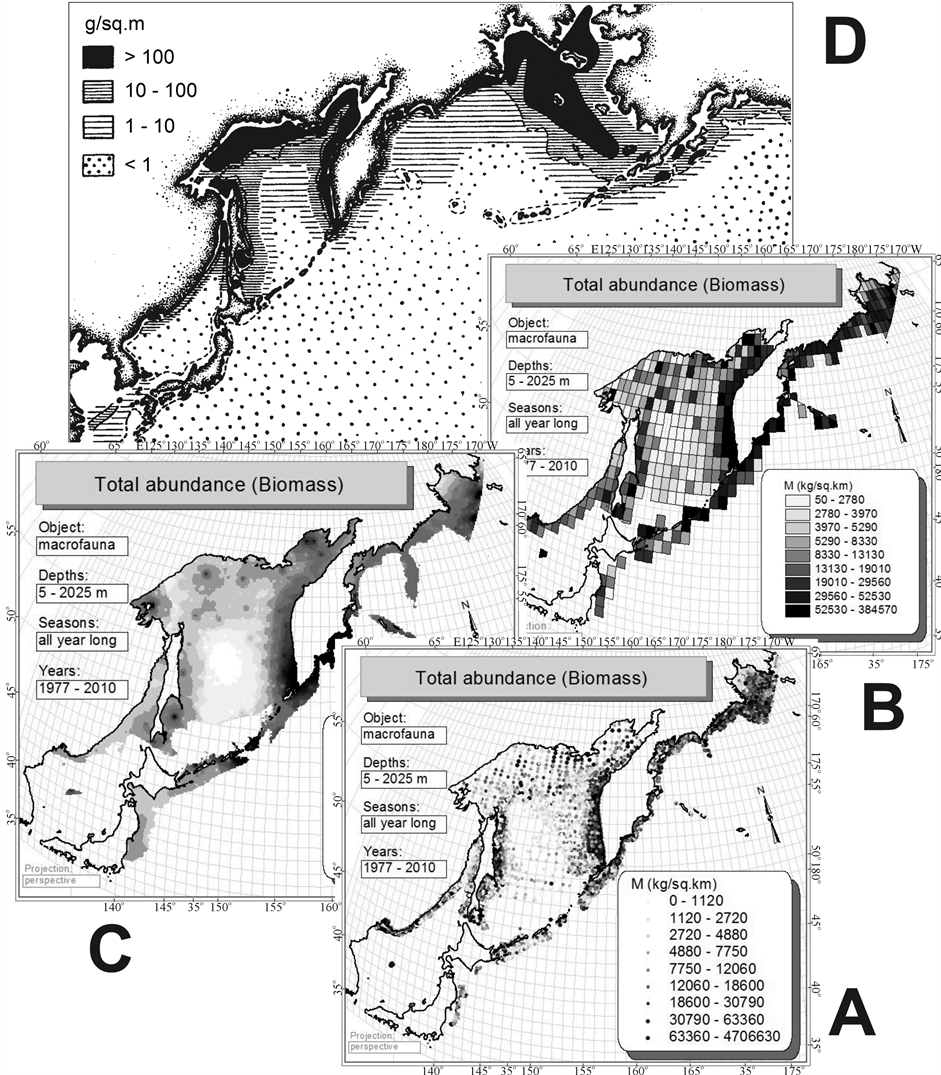
Figure 12. Horizontal distribution of benthic macrofauna biomass on bottom trawl stations (A), raster (B) and vector (C) maps of biomass distribution made from these data by averaging and interpolation. In the upper part of the figure for comparison given a map of benthos biomass distribution (D), obtained from the bottom grab samples data (From Ref. [58] ).
analogous patterns similar to what is known from the literature [58] on the distribution of biomass of benthos obtained from the bottom grab samples data in the Northern Pacific. It is reduced in the direction from the shores to the center of the ocean. By analogy, it should be assumed that the biomass of trawl macrofauna of benthal on the global level changes as it is shown in Figure 2(D), and, probably, in Figure 1(B). Such extrapolations can be made for species richness. Unfortunately, it is not yet possible to check them due to the lack of suitable bottom trawl systems.
In previous publications [35] -[37] , some additions were made to the Zenkevich-Bogorov’s concept of the biological structure of the ocean based on study results of pelagic macrofauna of this region:
When moving from the center of the Ocean to its periphery and in the direction of the depth to the surface water the stability of the environment conditions decreases and the intensity of water exchange intensity increases. Thereat, the environmental ecologic capacity grows up. Accordingly, the primary production and the biogeochemical cycle intensity increase in general. Also, the number, biomass and variations of average animals’ size, numerical and weighting prevalence of few dominant species over all others increase in the direction to the land. Thereat, the diversity decreases. Accordingly, the variability of population density and size of the animals, the dominance of mass species over others also increase with decreasing depth. However, the species richness and diversity decrease.
Having added to this the results of this article and having restated previous additions, one can come to the following conclusion.
5. Conclusions
Under the influence of the law of provincialism, the latitudinal zonality in the distribution of the integral characteristics of macrofauna is expressed extremely weakly in the northwestern Pacific, as against other regions. Here, the manifestation of circum-continental and vertical zonality predominates.
With increasing distance from the shore to the open sea and increasing depth the macrofauna abundance, as well as the variability of number, biomass, and average size of the animals and species richness go down. However, the average values of diversity and its components (species richness and evenness) decrease in the pelagial, and, at the bottom, the size of animals increases and the species richness decreases.
The species diversity and equitability near the bottom are correlated with the depth and distance from the land not uniquely. Probably, they are more dependent on local azonal factors: small-scale features of the bottom topography, soil, distribution of sediments and trophic zones.
The latest assumption can be checked only after digitizing the maps similar to those shown in Figures 11(B) and (C). This is a special challenge for the future and the subject of a separate publication.
References
- Zenkevich, L.A. (1948) The Biological Structure of the Ocean. Zoologicheskii Zhurnal, 27, 113-124.
- Bogorov, V.G. (1959) The Biological Structure of the Ocean. Doklady Akademii Nauk SSSR, 128, 819-822.
- Bogorov, V.G. (1970) The Biological Productivity of the Ocean and Features of Its Geographical Distribution. VoprosyGeografii, 84, 80-102.
- Bogorov, V.G. and Zenkevich, L.A. (1966) The Biological Structure of the Ocean. Ecology of Aquatic Organisms, Nauka Press, Moscow, 3-14.
- Humboldt, A. (1808) Ansichten der Naturmitwissenschaftlichen Erlauterungen. Cotta, Tubingen, 338 p.
- Wallace, A.R. (1878) Tropical Nature, and Other Essays. Macmillan, London, New York, 356 p. http://dx.doi.org/10.5962/bhl.title.1261
- Fischer, A.G. (1960) Latitudinal Variation in Organic Diversity. Evolution, 14, 64-81. http://dx.doi.org/10.1086/282398
- Pianka, E.R. (1966) Latitudinal Gradients in Species Diversity: A Review of Concepts. America/Natural, 100, 33-46. http://dx.doi.org/10.1086/282398
- Hillebrand, H. (2004) On the Generality of the Latitudinal Diversity Gradient. America/Natural, 163, 192-211. http://dx.doi.org/10.1086/381004
- Allen, A.P. and Gillooly, J.F. (2006) Assessing Latitudinal Gradients in Speciation Rates and Biodiversity at the Global Scale. Ecology Letters, 9, 947-954. http://dx.doi.org/10.1111/j.1461-0248.2006.00946.x
- Tittensor, D.P., Mora, C., Jetz, W., Lotze, H.K., Ricard, D., Berghe, E.V. and Worm, B. (2010) Global Patterns and Predictors of Marine Biodiversity across Taxa. Nature, 466, 1098-1103. http://dx.doi.org/10.1038/nature09329
- Bergmann, C. (1847) Ueber die Verhaltnisse der Warmeokonomie der Thierezuihrer Grosse. Gottinger Studien, 3, 595- 708.
- Lindsey, C.C. (1966) Body Sizes of Poikilotherm Vertebrates at Different Latitudes. Evolution, 20, 456-465. http://dx.doi.org/10.2307/2406584
- McDowal, R.M. (1994) On size and Growth in Freshwater Fish. Ecology of Freshwater Fish, 3, 67-79. http://dx.doi.org/10.1111/j.1600-0633.1994.tb00108.x
- Blackburn, T.M. and Gaston, K.J. (1996) Spatial Patterns in the Body Sizes of Bird Species in the New World. Oikos, 77, 436-446. http://dx.doi.org/10.2307/3545933
- Blackburn, T.M., Gaston, K.J. and Loder, N. (1999) Geographic Gradients in Body Size: A Clarification of Bergmann’s Rule. Diversity and Distributions, 5, 165-174. http://dx.doi.org/10.1046/j.1472-4642.1999.00046.x
- Ashton, K.G. (2004) Sensitivity of Intraspecific Latitudinal Clinic of Body Size for Tetrapods to Sampling, Latitude and Longitude? Integrative and Comparative Biology, 44, 403-412. http://dx.doi.org/10.1093/icb/44.6.403
- Watt, C. and Salewski, V. (2011) Bergmann’s Rule Encompasses Mechanism: A Reply to Olalla-Tarraga. Oikos, 120, 1445-1447. http://dx.doi.org/10.1111/j.1600-0706.2011.19968.x
- Bogorov, V.G. (1967) Biomass of Zooplankton and Productive Areas in the Pacific Ocean, Geographical Zonation of the Ocean. In: Biology of the Pacific Ocean, Part 1, Plankton, Nauka Press, Moscow, 221-227.
- Koblents-Mishke, O.I., Volkovinsky, V.V. and Kabanova, Yu.G. (1970) Plankton Primary Production of the World Ocean, Scientific Committee on Oceanographic Research (SCOR) Symp. Sci. Explor. South Pacific, National Academy of Science, Washington DC, 183-193.
- Moiseev, P.A. (1969) The Living Resources of the World Ocean. Pischevaya Promyshlennost Press, Moscow.
- Moiseev, P.A. (1977) Fishery Production of the World Ocean and Its Utilization, Oceanology: Ocean Biology [Online], In: Vol. 2. Biological Productivity of the Ocean, Nauka Press, Moscow, 289-314 (English Translation). http://www.archive.org/stream/ oceanologybiolog00nort/oceanologybiolog00nortdjvu.txt
- Shuntov, V.P. (1972) Seabirds and Biological Structure of the Ocean. Dalnevostochnoe KniznoyeIzdatelstvo Press, Vladivostok.
- Vinogradov, M.E. (1977) Oceanology. Ocean Biology. Vol. 1. Biological Structure of the Ocean. Nauka Press, Moscow.
- Zenkevich, L.A., Filatova, Z.A., Beliaev, G.M., Lukiyanova, T.A. and Suetova, I.A. (1971) Quantitative Distribution of the Zoobenthos in the World Ocean. Bull. Moip. Biol. Sect, 76, 27-33.
- Volvenko, I.V. (2007) Species Diversity of the Northwest Pacific Pelagic Macrofauna. Izv. TINRO, 149, 21-63.
- Volvenko, I.V. (2008) Species Diversity of Macrofauna Biomass in the Pelagic Northwest Pacific. Izv. TINRO, 153, 27-48.
- Volvenko, I.V. (2008) Species Richness of the Northwest Pacific Pelagic Macrofauna. Izv. TINRO, 153, 49-87.
- Volvenko, I.V. (2009) Species Structure Evenness of the Northwest Pacific Pelagic Macrofauna: 1. Number Equitability. Izv. TINRO, 156, 3-26.
- Volvenko, I.V. (2009) Species Structure Evenness of the Northwest Pacific Pelagic Macrofauna: 2. Biomass Equitability. Izv. TINRO, 156, 27-45.
- Volvenko, I.V. (2009) Abundance of the Northwest Pacific Pelagic Macrofauna: 1. Number. Izv. TINRO, 158, 3-39.
- Volvenko, I.V. (2009) Abundance of the Northwest Pacific Pelagic Macrofauna: 2. Biomass. Izv. TINRO, 158, 40-74.
- Volvenko, I.V. (2009) Average Individual Weight (Size) of Animals from Pelagic Macrofauna in the Northwest Pacific. Izv. TINRO, 158, 75-116.
- Volvenko, I.V. (2009) The Comparative Statuses of Far Eastern Seas and the Northwestern Pacific Based on the Range of Integral Characteristics of Pelagic Macrofauna. Russian Journal of Marine Biology, 35, 515-520. http://dx.doi.org/10.1134/S1063074009070013
- Volvenko, I.V. (2009) General Principles of Spatial-Temporal Variability of Integral Parameters for Pelagic Macrofauna in the Northwest Pacific. Izv. TINRO, 159, 43-69.
- Volvenko, I.V. (2009) General Patterns of Spatiotemporal Distribution of Pelagic Macrofauna Integrative Characteristics in the Northwest Pacific. Bulletin of the Far Eastern Brunch of the Russian Academy of Sciences, 3, 23-31.
- Volvenko, I.V. (2012) General Patterns of Spatial-Temporary Distribution of the Integral Characteristics of Pelagic Macrofauna of the North-Western Pacific and Biological Structure of Ocean. Journal of Earth Science and Engineering, 2, 1-14.
- Dontsova, Z.N. (1967) Sergey Semenovich Neustruev. Nauka, Moscow.
- Shannon, C.E. (1948) A Mathematical Theory of Communication. Bell System Technical Journal, 27, 379-423, 623-656.
- Margalef, R. (1958) Information Theory in Ecology. General Systems, 3, 36-71.
- McIntosh, R.P. (1967) An Index of Diversity and the Relations of Certain Concepts to Diversity. Ecology, 48, 392-404. http://dx.doi.org/10.2307/1932674
- Pielou, E.C. (1966) The Measurement of Diversity in Different Types of Biological Collections. Journal of Theoretical Biology, 13, 131-144. http://dx.doi.org/10.1016/0022-5193(66)90013-0
- Neyman, A.A., Zezina, O.N. and Semenov, V.N. (1977) Benthic Fauna of the Shelf and Continental Slope. Oceanology: Ocean Biology, Vol. 1, Nauka Press, Moscow, 269-281.
- Shuntov, V.P. (2001) Biology of Far-Eastern Seas of Russia. Vol. 1, TINRO-Center, Vladivostok, 580 p.
- Borets, L.A. (1997) Bottom Ichthyocenoses of the Russian Shelf of Far Eastern Seas: Composition, Structure, Elements of Functioning, and Commercial Importance. TINRO-Center, Vladivostok, 217 p.
- Kindlmann, P., Schodelbauerova, I. and Dixon, A.F.G. (2007) Inverse Latitudinal Gradients in Species Diversity. Scaling Biodiversity. Cambridge University Press, Cambridge, 246-257.
- Pyron, R.A. and Burbrink, F.T. (2009) Can the Tropical Conservatism Hypothesis Explain Temperate Species Richness Patterns? An Inverse Latitudinal Biodiversity Gradient in the New World Snake Tribe Lampropeltini. Global Ecology and Biogeography, 18, 406-415. http://dx.doi.org/10.1111/j.1466-8238.2009.00462.x
- Kiel, S. and Nielsen, S.N. (2010) Quaternary Origin of the Inverse Latitudinal Diversity Gradient among Southern Chilean Mollusks. Geology, 38, 955-958. http://dx.doi.org/10.1130/G31282.1
- Rivadeneira, M.M., Thiel, M., Gonzalez, E.R. and Haye, P.A. (2011) An Inverse Latitudinal Gradient of Diversity of Peracarid Crustaceans along the Pacific Coast of South America: Out of the Deep South. Global Ecology and Biogeography, 20, 437-448. http://dx.doi.org/10.1111/j.1466-8238.2010.00610.x
- Ashton, K.G., Tracy, M.C. and Quieroz, A. (2000) Is Bergmann’s Rule Valid for Mammals? American Naturalist, 156, 390-415. http://dx.doi.org/10.1086/303400
- Ashton, K.G. (2002) Do Amphibians Follow Bergmann’s Rule? Canadian Journal of Zoology, 80, 708-716. http://dx.doi.org/10.1139/z02-049
- Meiri, S. and Dayan, T. (2003) On the Validity of Bergmann’s Rule. Journal of Biogeography, 30, 331-351. http://dx.doi.org/10.1046/j.1365-2699.2003.00837.x
- Martof, B.S. and Humphries, R.L. (1959) Geographical Variation in the Wood Frog Rana sylvatica. American Midland Naturalist, 61, 350-389. http://dx.doi.org/10.2307/2422506
- Mayr, E. (1963) Animal Species and Evolution. Belknap Press Harvard University Press, Cambridge, xiv, 797 p.
- McNab, B.K. (1971) On the Ecological Significance of Bergmann’s Rule. Ecology, 52, 845-854. http://dx.doi.org/10.2307/1936032
- Gotthard, K. (2001) Growth Strategies of Ectothermic Animals in Temperate Environments. In: Atkinson, D. and Thorndyke, M., Eds., Animal Developmental Ecology. BIOS Scientific Publishers, Oxford, 287-304.
- Blanckenhorn, W.U. and Demont, M. (2004) Bergmann and Converse Bergman Latitudinal Clines in Arthropods: Two Ends of a Continuum? Integrative and Comparative Biology, 44, 413-424. http://dx.doi.org/10.1093/icb/44.6.413
- Neyman, A.A. (1965) Some Regularities of the Quantitative Distribution of Benthos on the North Pacific Shelves. Trudy Vsesoyuznogo Nauchno-Issledovatelskogo Instituta Morskogo Rybnogo Khozyaistva I Okeanografii, 57, 447-451.