Open Journal of Statistics
Vol.3 No.6(2013), Article ID:41534,8 pages DOI:10.4236/ojs.2013.36048
Robust Linear Regression Models: Use of a Stable Distribution for the Response Data
Medical School, University of São Paulo, Ribeirão Preto, Brazil
Email: *achcar@fmrp.usp.br
Copyright © 2013 Jorge A. Achcar et al. This is an open access article distributed under the Creative Commons Attribution License, which permits unrestricted use, distribution, and reproduction in any medium, provided the original work is properly cited. In accordance of the Creative Commons Attribution License all Copyrights © 2013 are reserved for SCIRP and the owner of the intellectual property Jorge A. Achcar et al. All Copyright © 2013 are guarded by law and by SCIRP as a guardian.
Received September 18, 2013; revised October 18, 2013; accepted November 18, 2013
Keywords: Stable Distribution; Bayesian Analysis; Linear Regression Models; MCMC Methods; OpenBugs Software
ABSTRACT
In this paper, we study some robustness aspects of linear regression models of the presence of outliers or discordant observations considering the use of stable distributions for the response in place of the usual normality assumption. It is well known that, in general, there is no closed form for the probability density function of stable distributions. However, under a Bayesian approach, the use of a latent or auxiliary random variable gives some simplification to obtain any posterior distribution when related to stable distributions. To show the usefulness of the computational aspects, the methodology is applied to two examples: one is related to a standard linear regression model with an explanatory variable and the other is related to a simulated data set assuming a 23 factorial experiment. Posterior summaries of interest are obtained using MCMC (Markov Chain Monte Carlo) methods and the OpenBugs software.
1. Introduction
A wide class of distributions that encompass the Gaussian distribution is given by the class of stable distributions. This large class defines location-scale families that are closed under convolution. The Gaussian distribution is a special case of this distribution family (see for instance, [1]), described by four parameters  and
and![]() . The
. The  parameter defines the “fatness of the tails”. When
 , this class reduces to Gaussian distributions. The
  is the skewness parameter and for
  one has symmetric distributions. The location and scale parameters are, respectively,
  and
and  (see [2]).
Stable distributions are usually denoted by . If a random variable
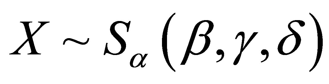 , then
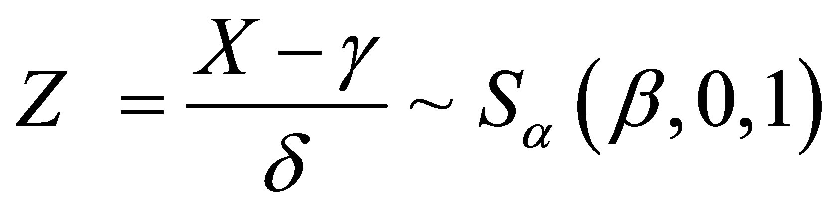
follows a standardized stable distribution (see [3] and [4]).
A great difficulty associated to stable distributions , is that in general there is no simple closed form for their probability density functions. However, it is known that the probability density functions of stable distributions are continuous ([5,6]) and unimodal ([7,8]). Also the support of all stable distributions is given in
 , except for
  and
and  when the support is
  for
for  and
and  for
for  (see [9]).
The characteristic function  of a stable distribution is given by,
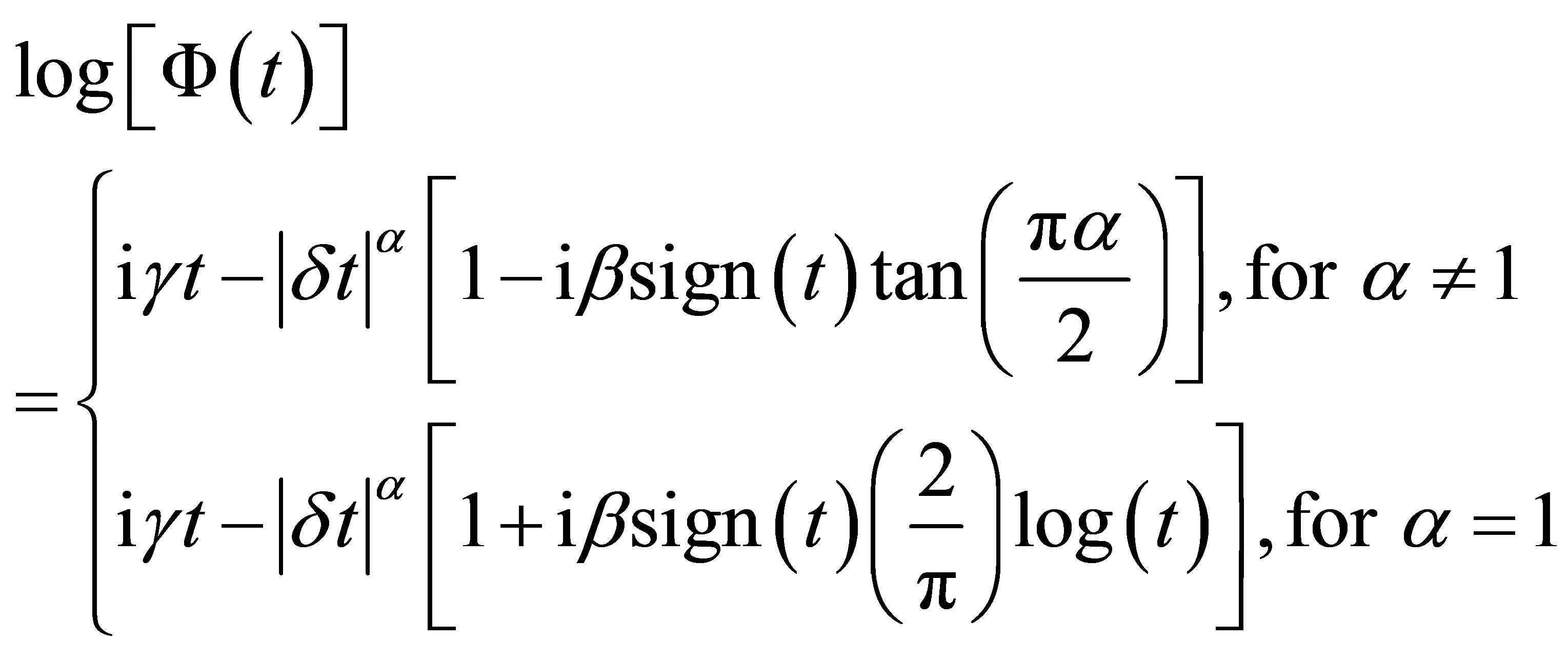 (1.1)
(1.1)
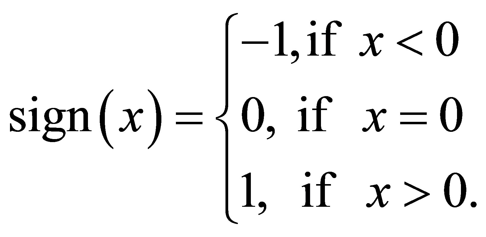
where  and sign (.) function is given by
It is important to point out that if , the variance is infinite and the mean of the stable distribution does not exist.
Although this class of distributions is a good alternative for data modeling in different areas, we usually have difficulties to obtain estimates under a classical inference approach due to the lack of closed form expressions for their probability density functions. One possibility in applications is to get the probability density function from the inversion formula (see, for example [10]),
 , (1.2)
where  is the characteristic function. In applications, we need use numerical methods to solve the integral in (1.2), usually taking a great computational time.
An alternative is the use of Bayesian methods. However, the computational cost can be further high to get the posterior summaries of interest. A good alternative is to use latent or artificial variables that could improve the simulation computation of samples of the joint posterior distributions of interest (see, for example [11,12]).
In this way, a Bayesian analysis of stable distributions was introduced by [1] using Markov Chain Monte Carlo (MCMC) methods and latent variables (see also, [13]). The use of Bayesian methods with MCMC simulation can have great flexibility by considering latent variables where samples of latent variables are simulated in each step of the Gibbs or Metropolis-Hastings algorithms(see for example [14,15]).
Considering a latent or an auxiliary variable, [1] proved a theorem that is useful to simulate samples of the joint posterior distribution for the parameters  and
and![]() . This theorem establishes that a stable distribution for a random variable Z defined in
. This theorem establishes that a stable distribution for a random variable Z defined in  is obtained as the marginal of a bivariate distribution for the random variable Z itself and an auxiliary random variable Y. This variable Y is defined in the interval
 , when
 , and in
 , when
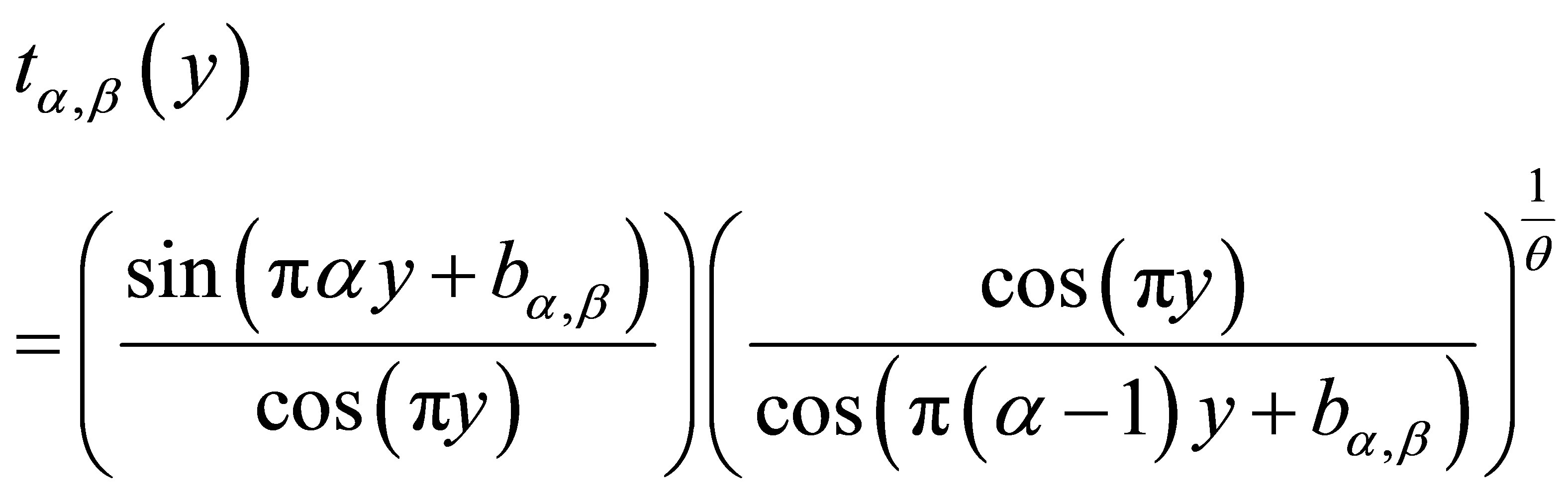
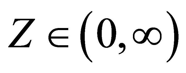 . The quantity
  is given by
 (1.3)
(1.3)
where 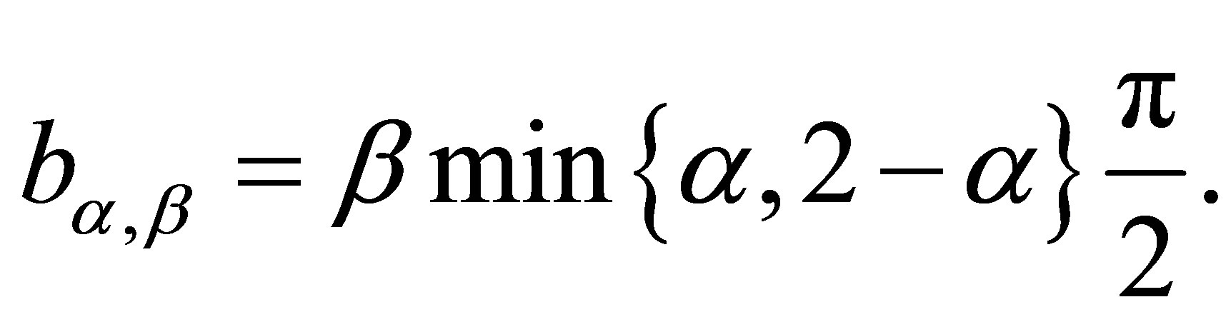
The joint probability density function for random variables Z and Y is given by
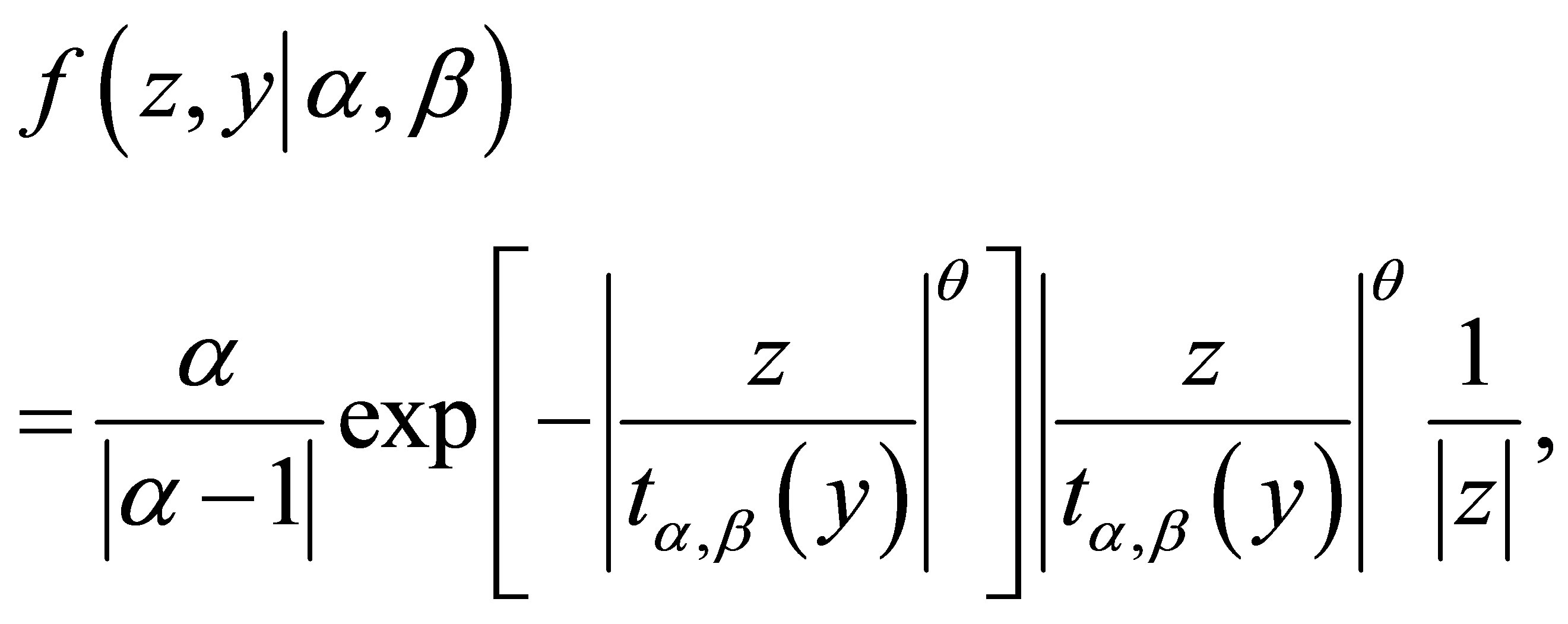 (1.4)
(1.4)
where 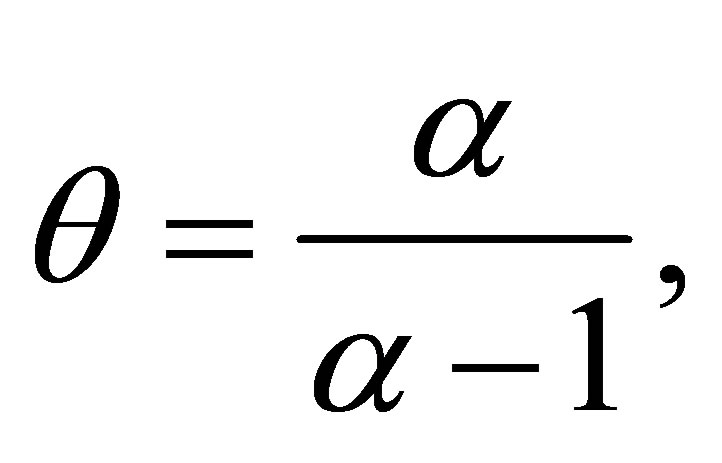
 (1.5)
(1.5)
and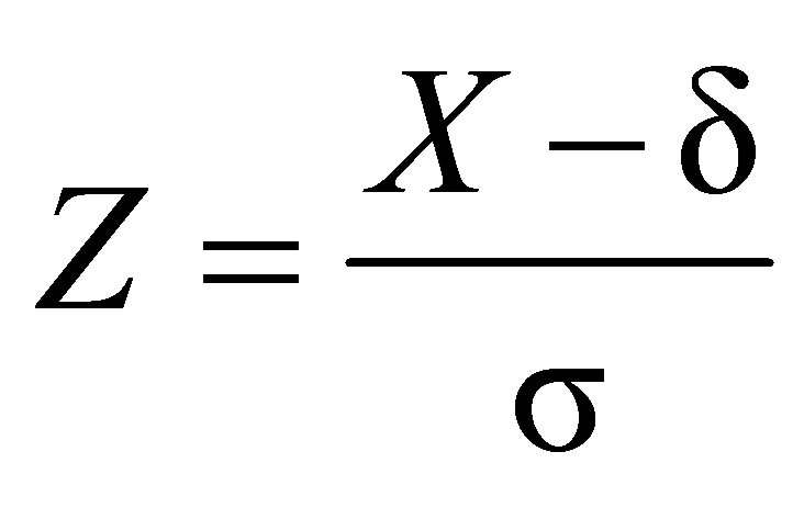 , for
, for 
From the bivariate density (1.4), [1] showed the marginal distribution for the random variable Z is stable  (
( , 0, 1) distributed. Usually, the computational costs to obtain posterior summaries of interest using MCMC methods are high for this class of models, which could give some limitations for practical applications. One problem can be the simulation algorithm convergence. In this paper, we propose the use of the popular free available software to obtain the posterior summaries of interest: the OpenBUGS software.
The paper is organized as follows: in Section 2, we introduce linear regression models assuming a stable distribution; in Section 3, we introduce a Bayesian analysis for linear regression models assuming a stable distribution; in Section 4, we present two examples to illustrate the proposed methodology; finally, in Section 5, we present some concluding remarks.
2. Linear Regression Models Assuming a Stable Distribution
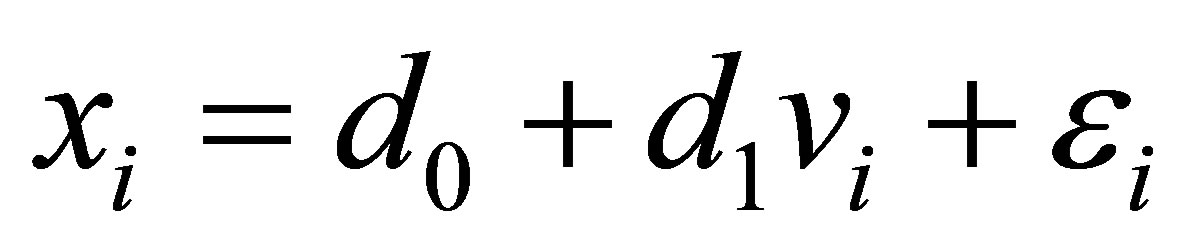
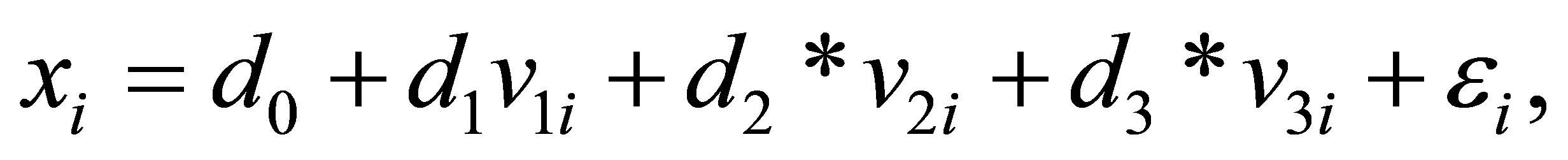
Consider a random variable X related to a controlled variable v given by the linear relationship,
 , (2.1)
for , where1) The random variable
  represents the response for the i-th unit associated with an experimental value of the independent or explanatory variable vi assumed as a fixed value. In this way, xi is an observation of Xi.
2) The variables  are considered as components of unknown errors as unobserved random variables. Assume that these random variables
 ![]() are independent and identically distributed with normal distribution
are independent and identically distributed with normal distribution .
.
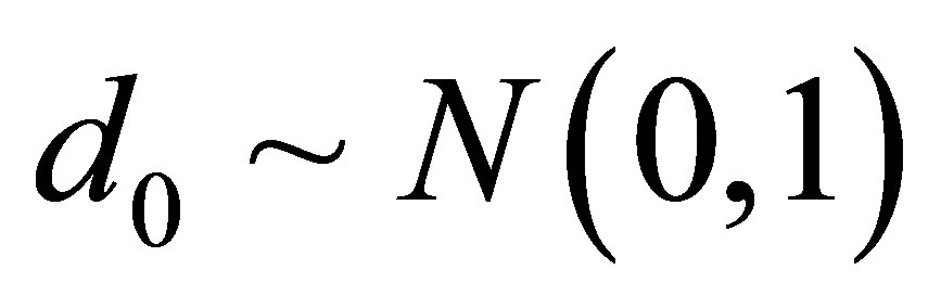
3) The parameters d0 and d1 are unknown.
From the above assumptions, we have normality for the responses, that is,
 . (2.2)
In this way Xi has a normal distribution with mean  and common variance
 .
.
Usually we get estimators for the regression parameters using minimum squares approach or standard maximum likelihood methods (see for example, [16,17]).
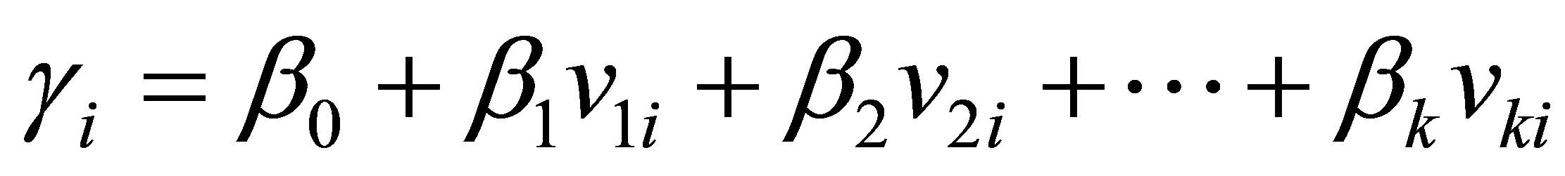
Standard generalization for the linear model (2.1) is given in presence of k independent or explanatory variables, that is, a multiple linear regression model, given by,
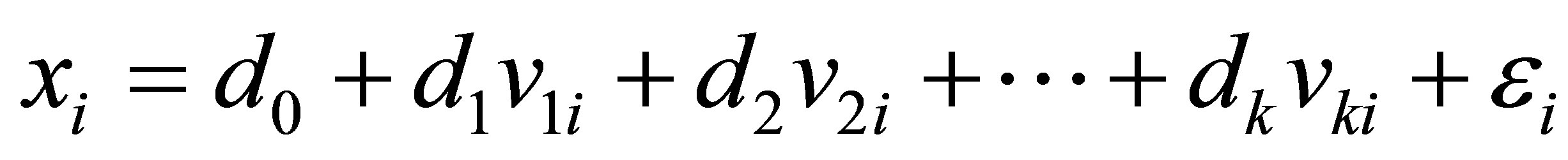 . (2.3)
From the normality assumption for the error ei in (2.3), the random variable Xi has a normal distribution with mean 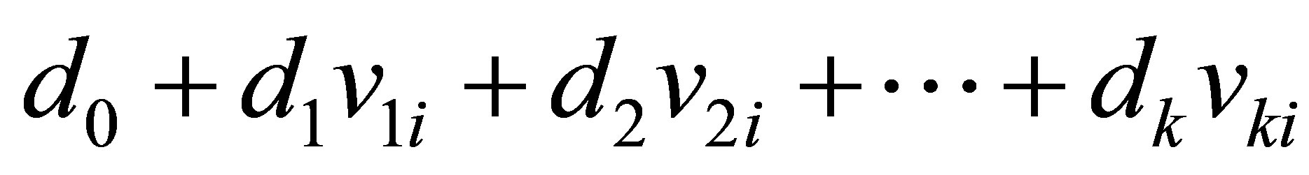 and variance
 .
.
In practical work, in all applications we need to check if the above assumptions are verified. In this way, we consider graphical approaches to verify if the residuals of the model satisfy the above assumptions.
In presence of outliers or discordant observations we could have great effects on the obtained estimators for the regression model given by (2.3) which could invalidate the obtained inferences. In this way, we could use nonparametric regression models or to assume more robust probability distributions for the data. One possibility is to assume that the random variable X in (2.3) or (2.1) have a stable distribution .
.
3. A Bayesian Analysis for Linear Regression Models Assuming a Stable Distribution
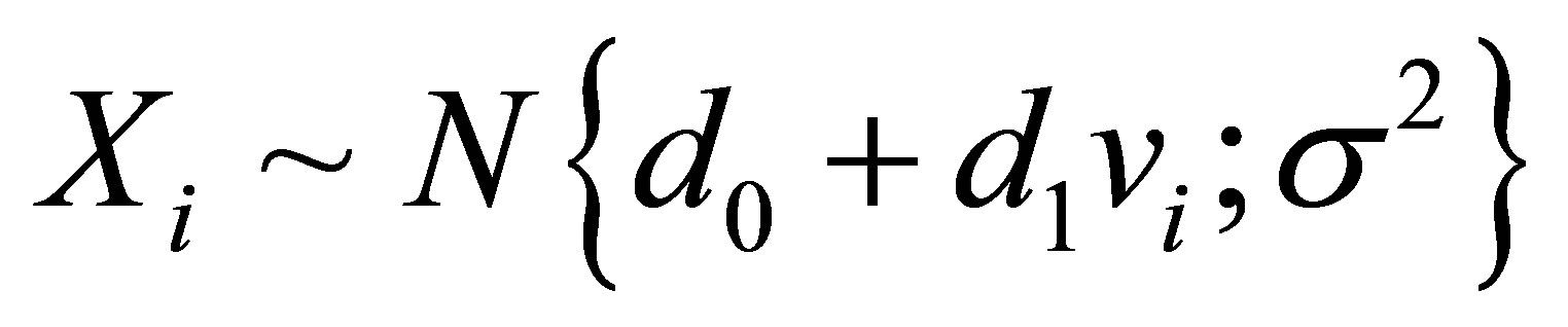
In this section, let us assume that the response xi in the linear regression model (2.3) for , have a stable distribution
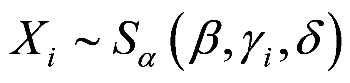 , that is,
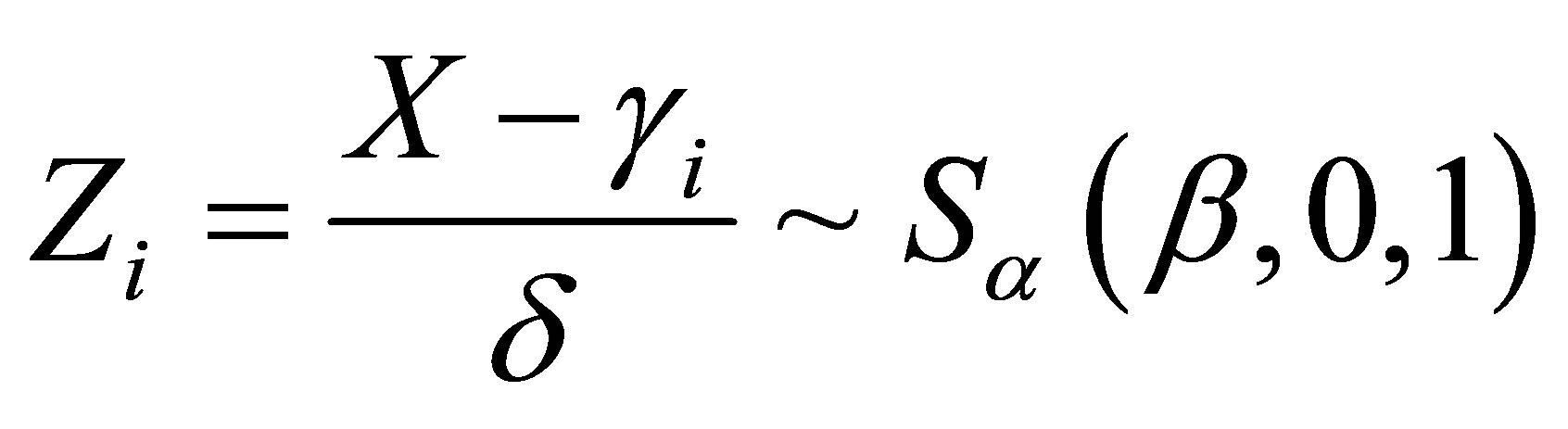
and where the location parameter  of the stable distribution is related to the explanatory variables by a linear relation given by,
 . (3.1)
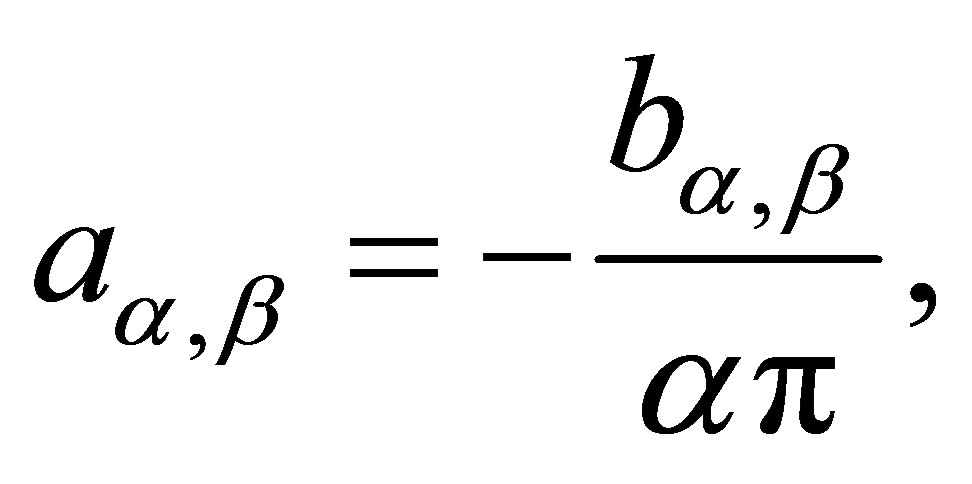
Assuming a joint prior distribution for α, β, d and δ, where  given by
 , [1] shows that the joint posterior distribution for parameters α, β, d and δ, is given by,
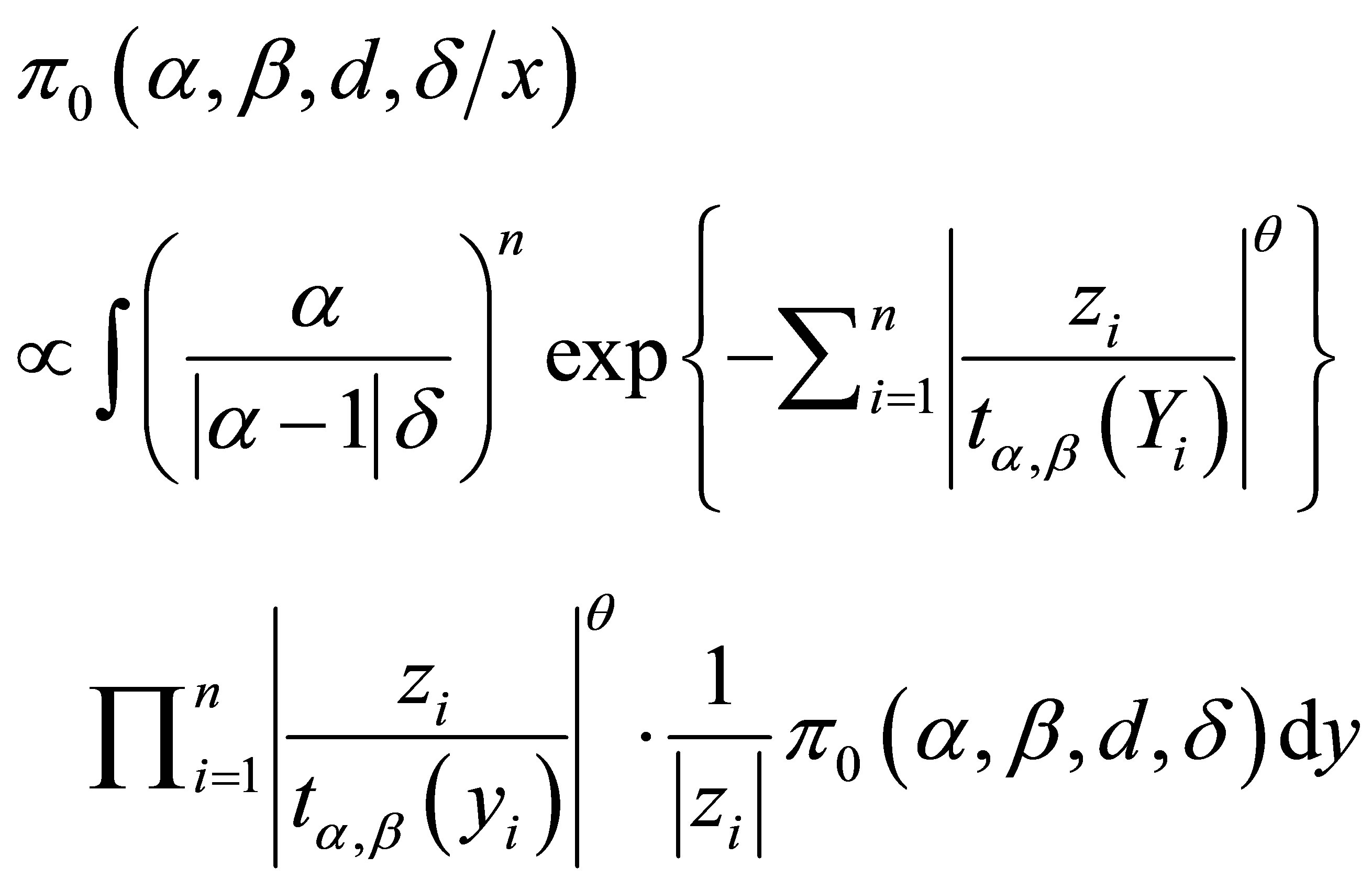 (3.2)
(3.2)
where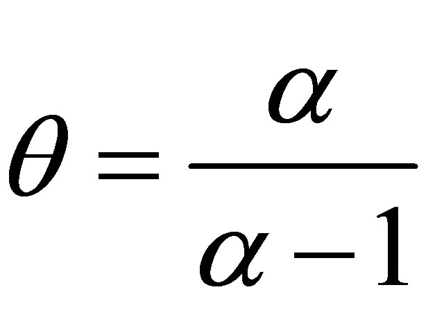 ,
,  , for
, for ,
,  ,
,
 and
and ;
;  and
and  are respectively, the observed and non-observed data vectors. Observe that the bivariate distribution in expression (3.2) is given in terms of
  and the latent variables
 , and not in terms of
 ![]() and
and  (there is the Jacobian
  multiplied by the right-handside of expression (1.4)).
Observe that when  we have
  and
and . In this case we have a Gaussian distribution with mean equals to δ and variance equals to
 .
.
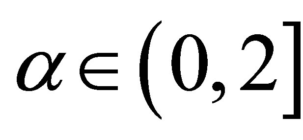
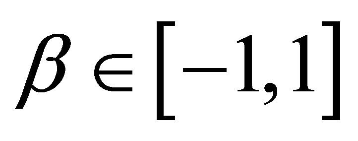
For a Bayesian analysis of the proposed model, we assume uniform  priors for
  where the hyperparameters a and b are assumed to be known in each application following the restrictions
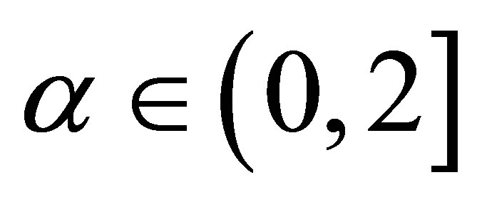 ,
,
 and
and . We also assume Normal
 prior distributions for the regression parameters
  considering known hyperparameter values a and b2. We further assume independence among all parameters.
In the simulation algorithm to obtain a Gibbs sample for the random quantities α, β, d and δ, having the joint posterior distribution (3.2), we assume a uniform  prior distribution for the latent random quantities
 ![]() for
for  Observe that, in this case, we are assuming
 . With this choice of priors, we use standard available software packages like OpenBugs (see [18]) which gives great simplification to obtain the simulated Gibbs samples for the joint posterior distribution of interest.
From expression (3.2), the joint posterior probability distribution for and
and  is given by,
 (3.3)
(3.3)
where  and
and  are respectively defined in (1.4)
and (1.5) and  is a
is a  density function, for
 .
.
Since we are using the OpenBugs software to simulate samples for the joint posterior distribution we do not present here all full conditional distributions needed for the Gibbs sampling algorithm. This software only requires the data distribution and prior distributions of the interested random quantities.
This gives great computational simplification for determining posterior summaries of interest as shown in the applications as follows.
In these applications we illustrate the proposed methodology to real and simulated data sets, in special, showing the robustness of the model in presence of outliers.
4. Some Applications
4.1. An Example with a Simple Linear Regression Model
In Table 1, we have a data set related to an industrial experiment, where x denotes the response and v denotes an explanatory variable associated to each response (n = 15 observations).
From a preliminary data analysis, we see that a linear regression model (2.1) is suitable for the data set. The estimated regression straight line obtained by minimum squares estimates and using the software MINITAB version 16 is given by 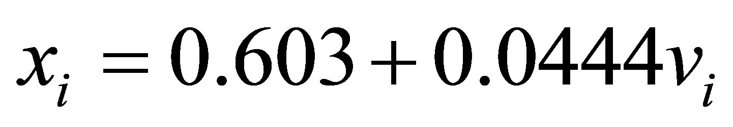 where the regression parameter d1 is statistically different of zero (p-value < 0.05). From standard residuals plots we verify that the required assumptions (normality of the residuals and constancy of the variance are verified).
Under a Bayesian approach, we have in Table 2, the posterior summaries of interest assuming the linear regression model defined by (3.1) with a stable distribution for the response and the OpenBugs software assuming the following prior distributions: ,
,  ,
,  ,
,  and
and . We also assume a uniform
  distribution for the latent variable Yi,
 . We simulated 800,000 Gibbs samples, with a “burn-in-sample” of 300,000 samples discarded to eliminate the effects of the initial values in the iterative simulation process and taking a final sample of size 1,000 (every 500th sample chosen from the
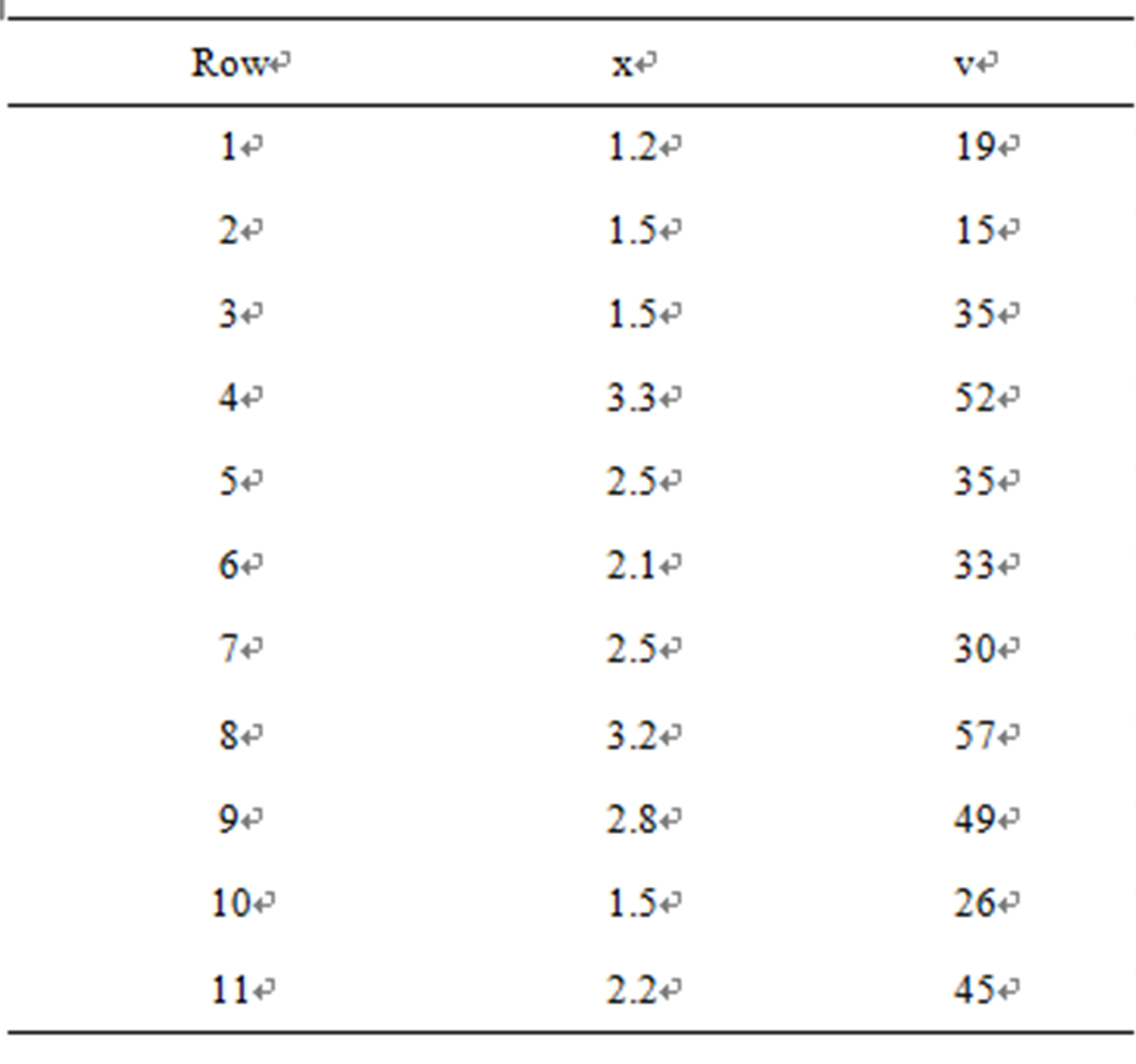
Table 1. An industrial experiment data set.
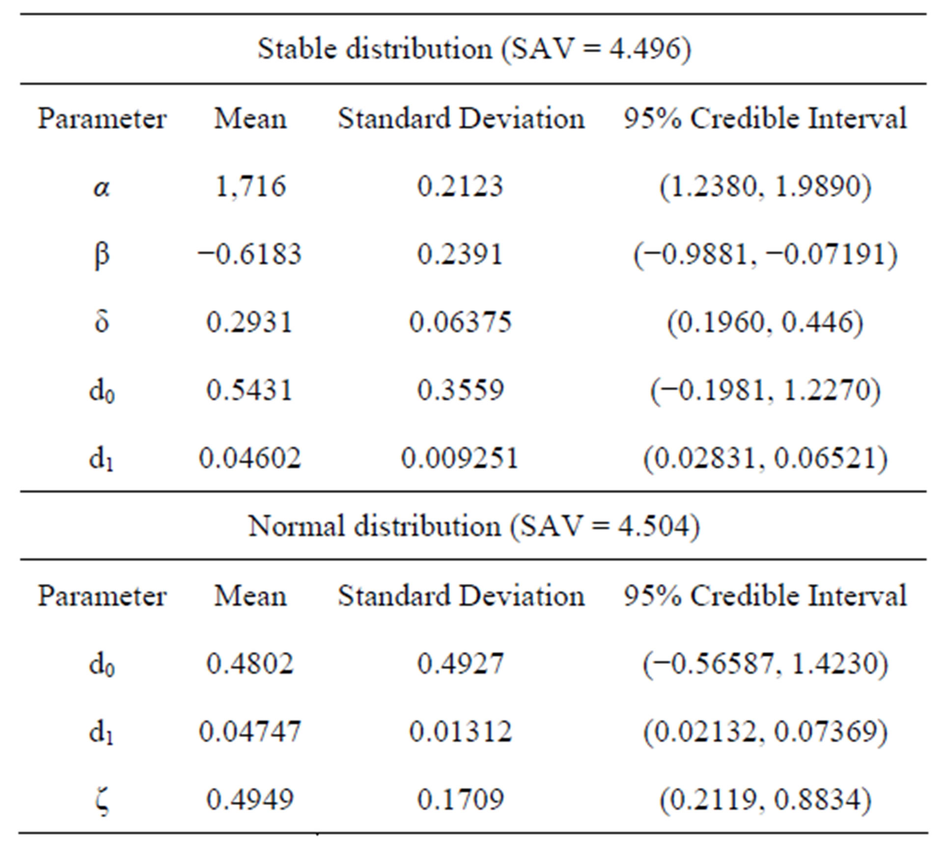
Table 2. Posterior summaries (linear regression).
500,000 samples). Convergence of the Gibbs sampling algorithm was monitored from standard trace plots of the simulated samples.
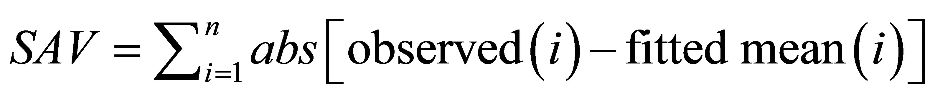
In Table 2, we also have the sum of absolute values between (SAV) the observed and fitted values, given by,
 (4.1)
(4.1)
In Table 2, we also have the posterior summaries of the regression model (2.1) assuming a normal 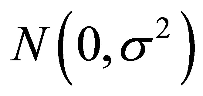 distribution for the error and the following priors for the parameters of the model:
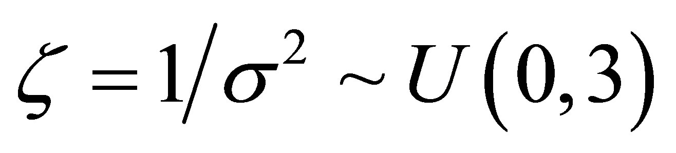 ,
,  and
and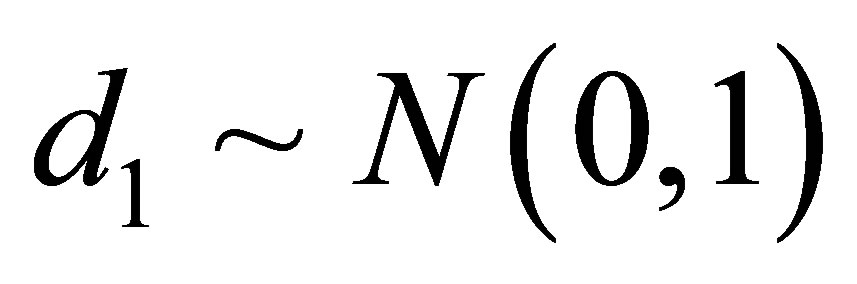 . In this case, we simulated 55,000 Gibbs samples taking a “burn-in-sample” of size 5,000 using the OpenBugs software. From the results of Table 2, we observe similar results assuming normality or a stable distribution for the data. In this case, we conclude that we do not need to assume a stable distribution for the data, since the results are very similar assuming usual normality for the errors and the computational cost using stable distributions is very high.
In Figure 1, we have the plots of observed, fitted means considering both models versus samples. From the plots of Figure 1, we observe similar fit of both models (linear regression model assuming normality or a stable distribution). Observe that we have SAV = 4.496 assuming a stable distribution and SAV = 4.504 assuming a normal distribution, that is, very close results.
Now let us consider the presence of an outlier or discordant response (considered as a measure error) replacing the 15th response (2.8) in Table 1 by the value 8.0 (denoted as outlier 1). In Table 3, we have the obtained posterior summaries assuming the same priors and simulation procedure assumed for the results of Table 2. In Figure 2, we have the plots of observed, fitted means
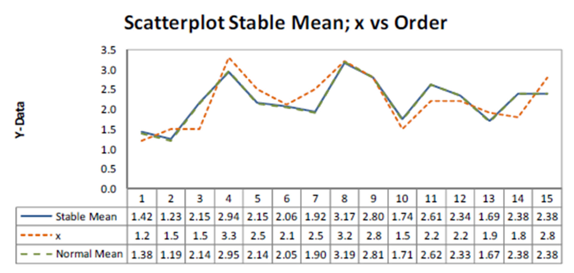
Figure 1. Plots of observed, fitted means considering both models versus samples.
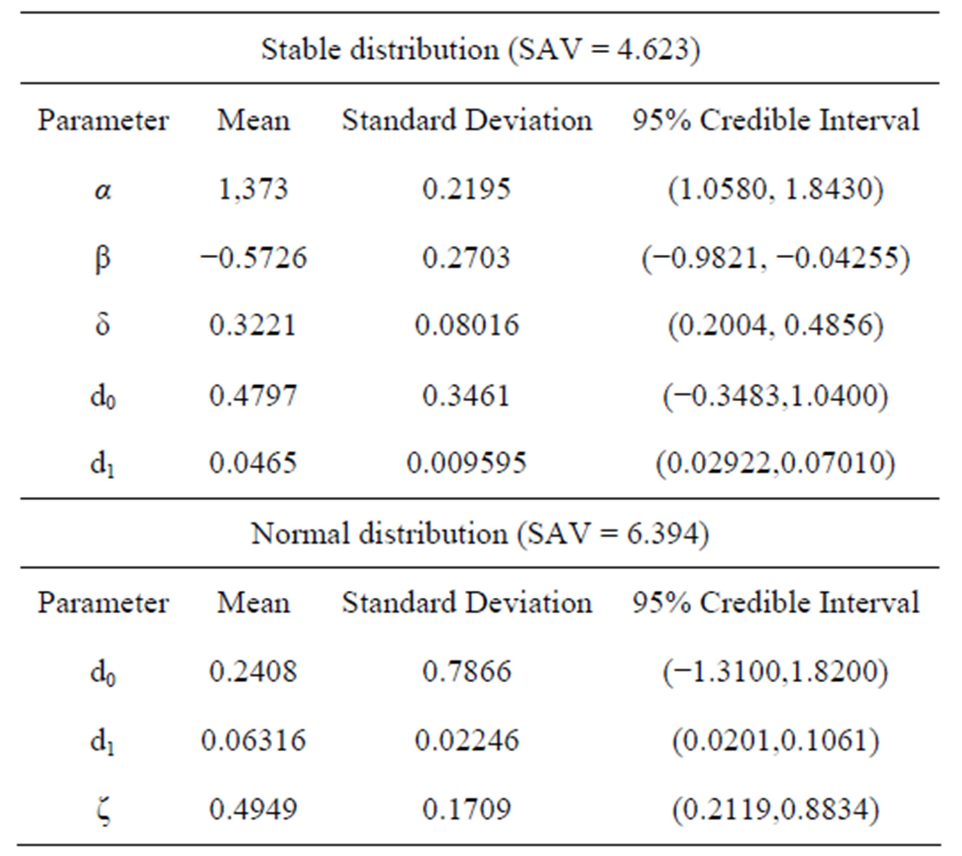
Table 3. Posterior summaries (example 1, with outlier 1).
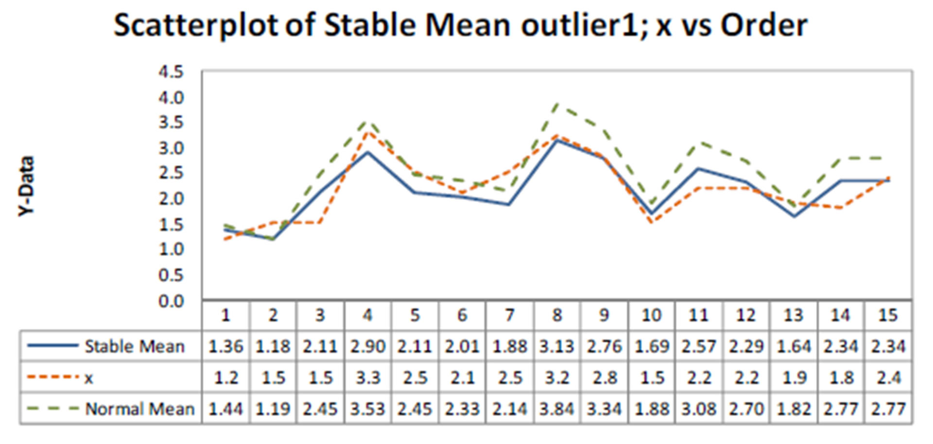
Figure 2. Plots of observed, fitted means considering both models (presence of outlier 1).
considering both models versus samples. From the plots of Figure 2, we observe that model with a stable distribution is very robust to the presence of the outlier given similar inference results as obtained without the presence of the outlier (see results in Table 2). We also observe in Table 3, that the estimated regression parameters with normal error are strongly affected by the presence of the outlier 1. Observe that we have SAV = 4.623 assuming a stable distribution (a value very close to the SAV values given in Table 2, without the presence of an outlier) and SAV = 6.394 assuming a normal distribution.
Similarly, we have in Table 4 the posterior summaries assuming another outlier replacing the 15th response (2.8) in Table 1 by the value 50.0 (denoted as outlier 2). In Figure 3, we have the plots of observed, fitted means considering both models versus samples for this case.
From the plots of Figure 3, we observe that model with a stable distribution is very robust to the presence of outliers even considering a large discordant observation (outlier 2). We also observe in Table 4, that the estimated regression parameters of regression model with normal error are strongly affected by the presence of the outlier 2. Observe that we have SAV = 4.632 assuming a stable distribution (a value very close to the values given in Table 2, without the presence of an outlier) and SAV = 46.083 assuming a normal distribution, that is, with very large values of outliers the obtained inferences are greatly affected assuming normality for the data.
4.2. An example with Simulated Data (5 Replicates of a Factorial 23 Experiment)
In Table 5, we have 40 responses simulated from a factorial 23 experiment with 5 replicates assuming the
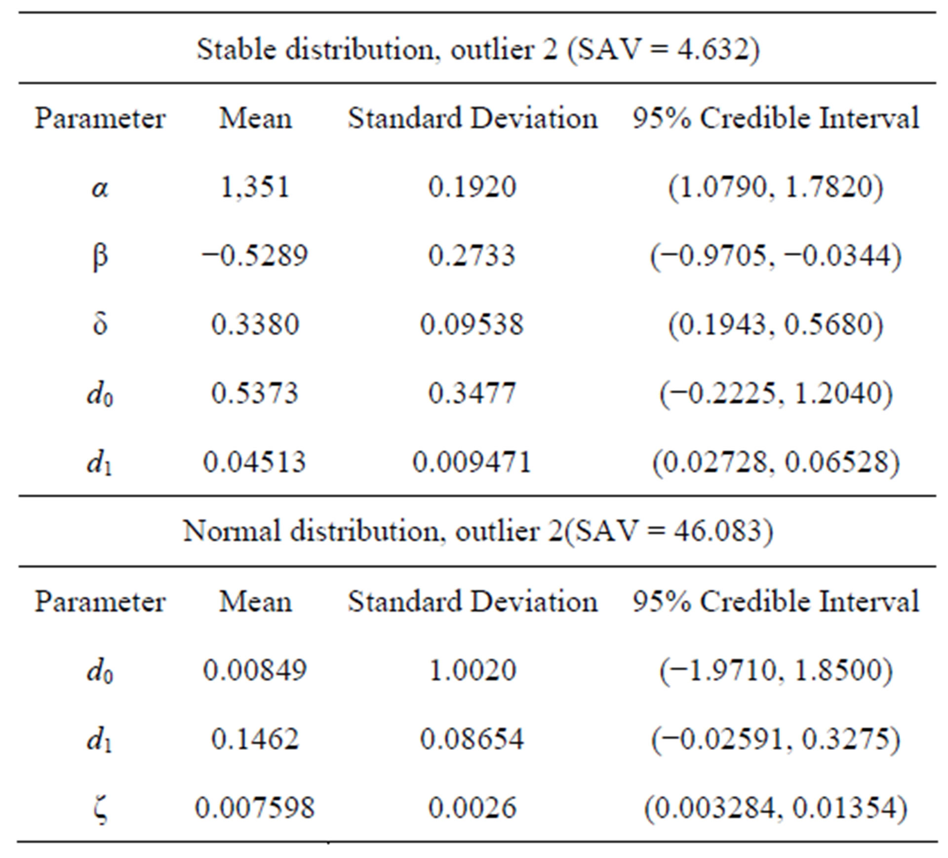
Table 4. Posterior summaries (example 1, with outlier 2).
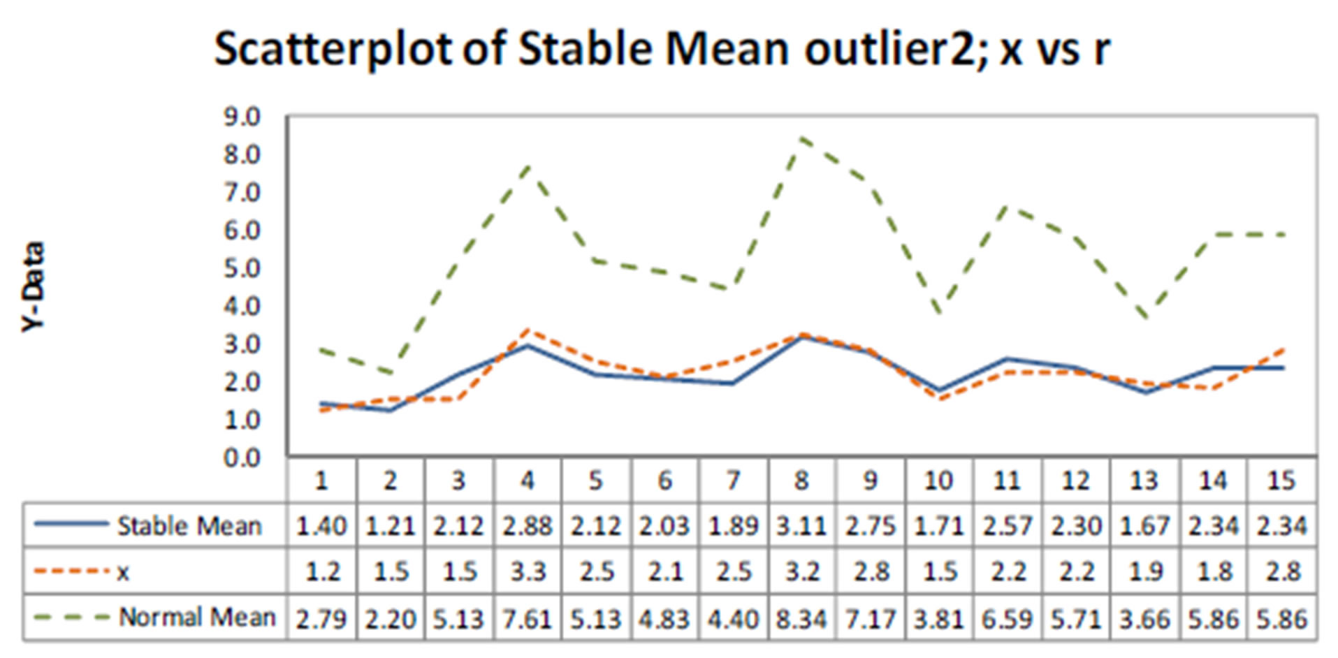
Figure 3. Plots of observed, fitted means considering both models (presence of outlier 2).
following model,
 , (4.2)
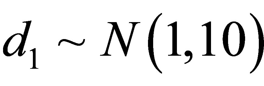
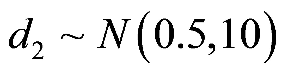
where d0 = 2, d1 = 1, d2 = 0.5, d3 = 1.8 and ei are independent and identically distributed errors with a normal distribution N (0, 1).
The estimated regression obtained by minimum squares estimates and using the software MINITAB version 16 is given by xi = 2.19 + 0.964v1i + 0.828v2i + 2.08v3i where the regression parameters d1, d2, and d3 are statistically different of zero (p-value < 0.05 for all regression parameters). From standard residuals plots we verify that the required assumptions (normality of the residuals and constancy of the variance are verified).
Under a Bayesian approach, we have in Table 6, the posterior summaries of interest assuming the linear regression model defined by (3.1) with a stable distribution for the response and the OpenBugs software assuming the following prior distributions: ,
,  ,
,  ,
,  and
and ,
,  ,
,  and
and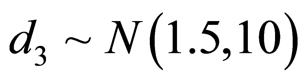 .We also assume a uniform
  distribution for the latent variable Yi,
 . We simulated 400,000 Gibbs samples, with a “burn-in-sample” of 100,000 samples discarded to eliminate the effects of the initial values in the iterative simulation process and taking a final sample of size 1,500 (every 200th sample chosen from the 300,000 samples). Convergence of the Gibbs sampling algorithm was monitored from standard trace plots of the simulated samples. From the results of Table 6, we observe that the parameter α has a Monte Carlo estimate for the posterior mean for α given by 0.9089, that is, the mean of the stable distribution is not defined in this case (α < 1).
In Table 6, we also have the posterior summaries of the regression model (4.2) assuming a normal  distribution for the error and the following priors for the parameters of the model:
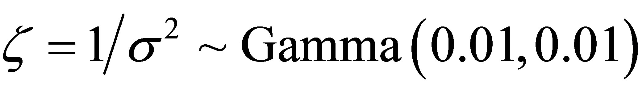 , where Gamma
  denotes a gamma distribution with mean
  and variance
 ,
,  ,
,  ,
,  and
and . In this case, we simulated 55,000 Gibbs samples taking a “burn-in-sample” of size 5,000 using the OpenBugs software. From the results of Table 6, we observe similar results for the Bayesian estimates of the regression parameters assuming normality or a stable distribution for the data.
Now let us assume the presence of an outlier or discordant response (measure error) replacing the 30th response (5.04875) in Table 5, by the value 25.250. In Table 7, we have the obtained posterior summaries assuming the same priors and simulation procedure assumed for the results of Table 6. We observe in Table 7, that the estimated regression parameters assuming normal error are strongly affected by the presence of the outlier.
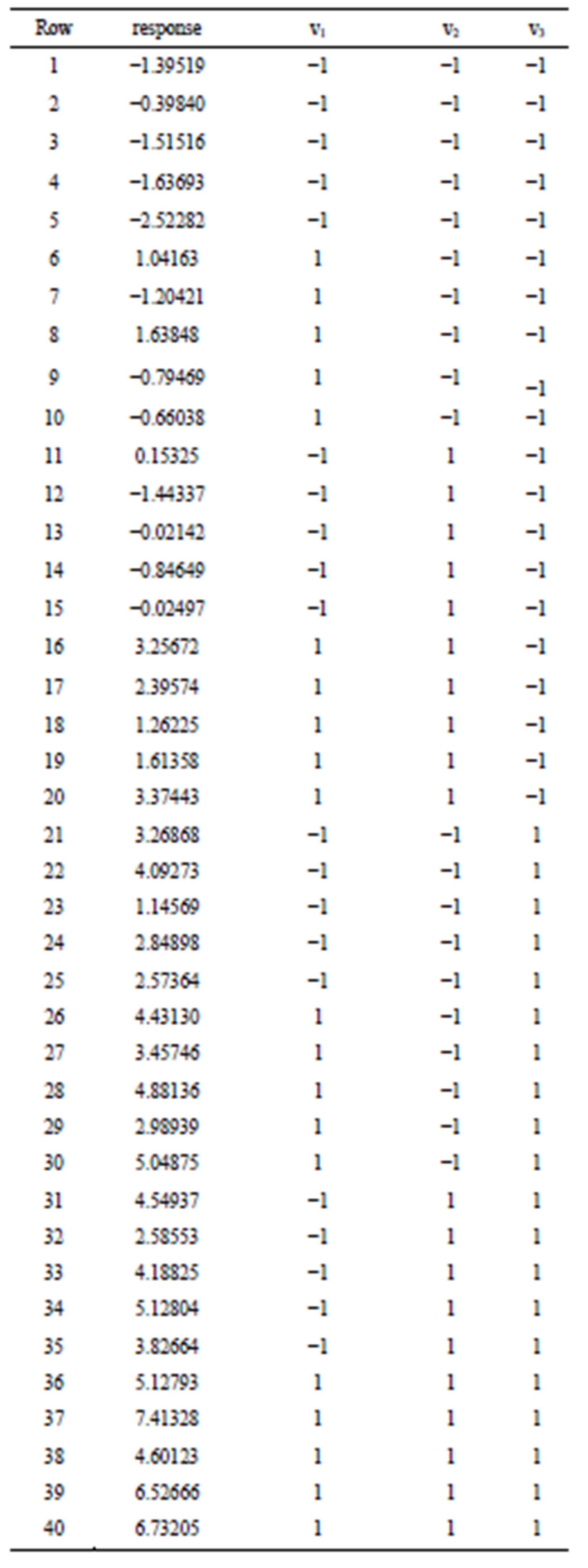
Table 5. A simulated data set.
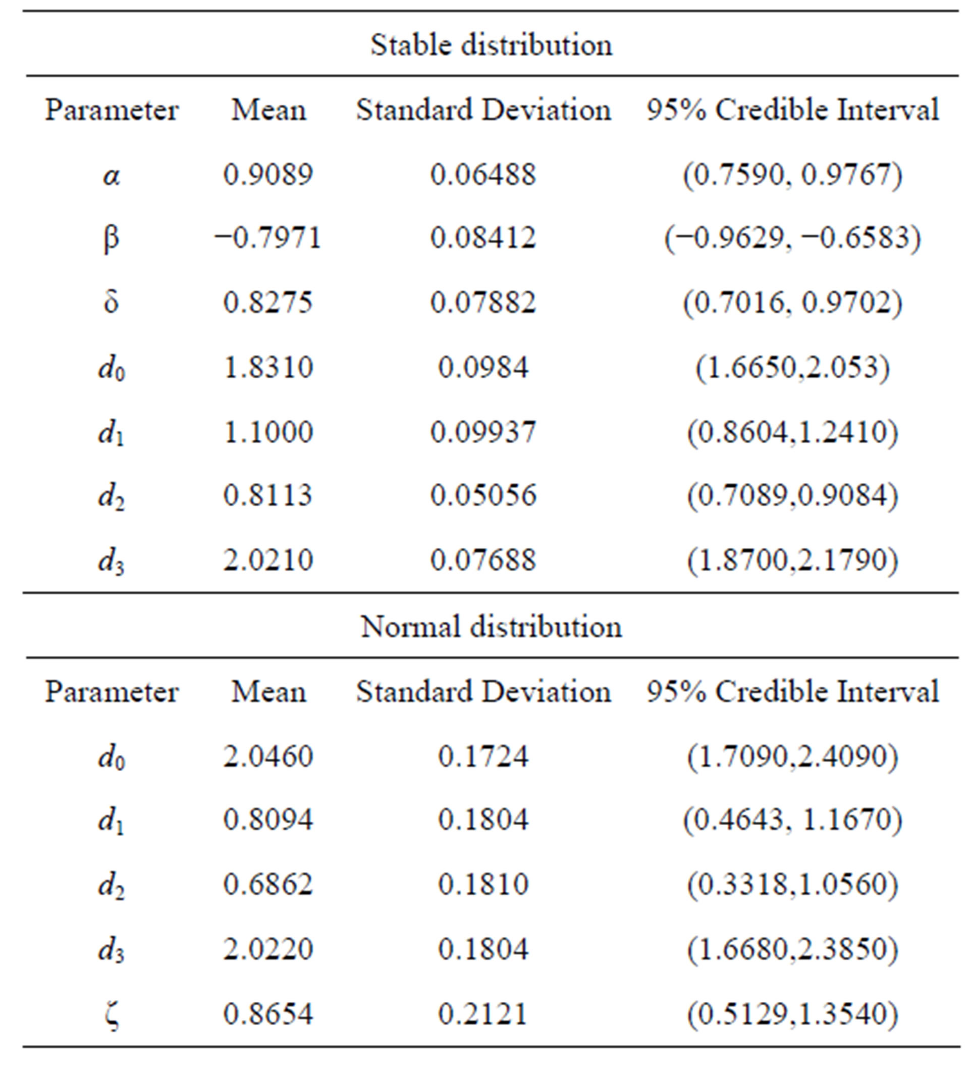
Table 6. Posterior summaries (simulated data).
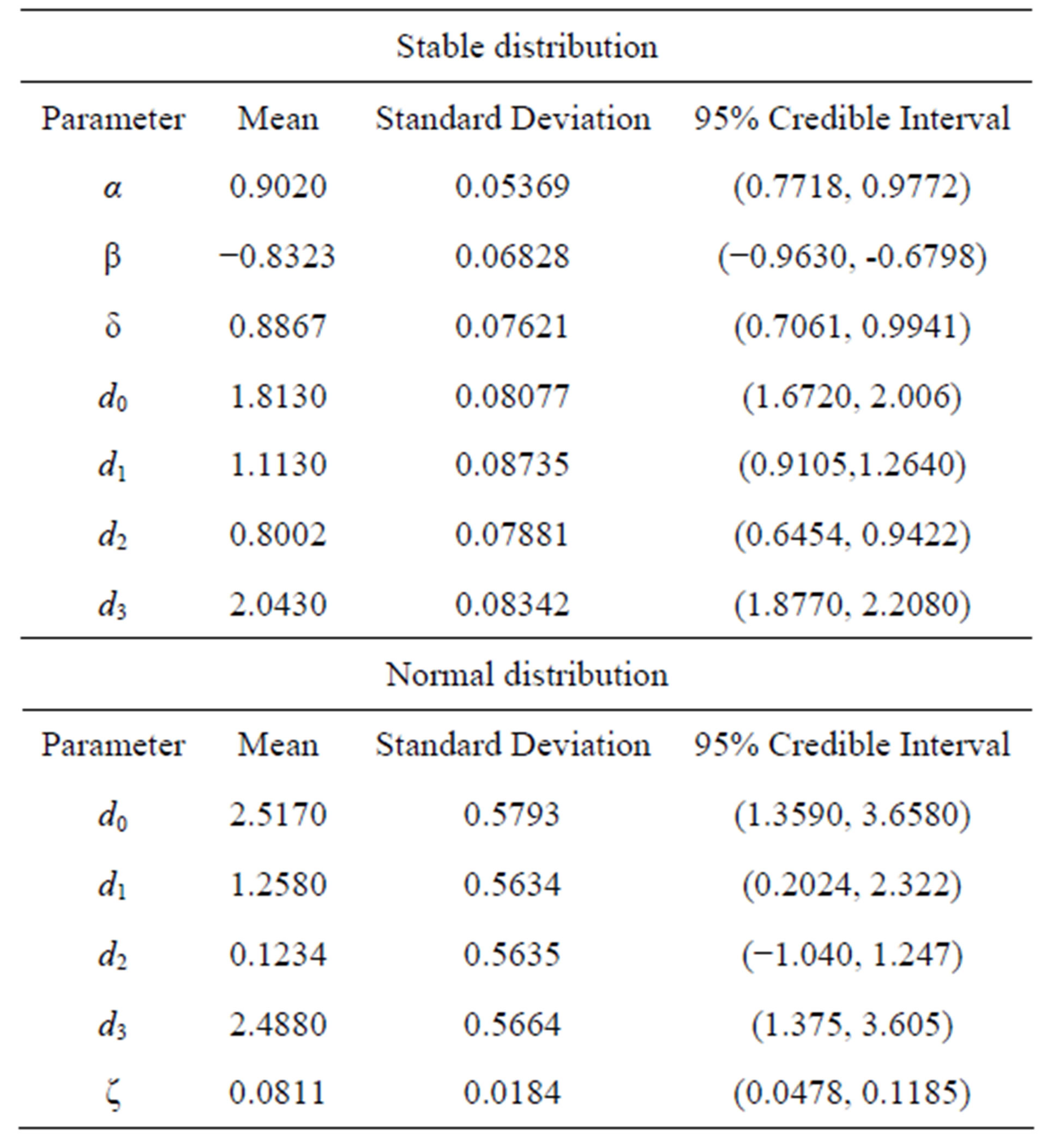
Table 7. Posterior summaries (simulated data in the presence of an outlier).
5. Concluding Remarks
The presence of outliers or discordant observations is due to the measure errors many times. This situation is very common in applications of the regression analysis. In the presence of these discordant observations, the usual obtained inferences on the regression parameters or in the predictions based on minimum squares approach or maximum likelihood approach under the usual assumption of normality for the errors and constant variance could be greatly affected, which could imply in wrong inference results. The use of stable distributions could be a good alternative for many applications in the data analysis to have robust inference results, since this distribution has a great flexibility to fit for the data. With the use of Bayesian methods and MCMC simulation algorithms, it is possible to get inferences for the model despite of the nonexistence of an analytical form for the density function as it was showed in this paper. It is important to point out that the computational work in the sample simulations for the joint posterior distribution of interest can be greatly simplified using standard free softwares like the OpenBugs software.
Observe that in general, the appearance of outliers will absolutely affect the regression model under standard normality assumptions. The ideal results not affected by outliers could be obtained using the proposed methodology as observed in our applications. These results could be of great interest in applications.
In both examples introduced in Section 4, the use of data augmentation techniques (see, for instance, [11]) is the key to obtain a good performance for the MCMC simulation method for applications using stable distributions.
We emphasize that the use of OpenBugs software does not require large computational time to get the posterior summaries of interest, even when the simulation of a large number of Gibbs samples is needed for the algorithm convergence. These results could be of great interest for researchers and practitioners, when dealing with nonGaussian data, as in the applications presented here.
6. Acknowledgements
J. A. Achcar and E. Z. Martinez gratefully acknowledge the financial support from the Brazilian Institution Conselho Nacional de Desenvolvimento Científico e Tecnológico (CNPq).
REFERENCES
- D. J. Buckle, “Bayesian Inference for Stable Distributions,” Journal of the American Statistical Association, Vol. 90, 1995, pp. 605-613. http://dx.doi.org/10.1080/01621459.1995.10476553
- P. Lévy, “Théorie des Erreurs la loi de Gauss et les Lois Exceptionelles,” Bulletin Society Mathematical, Vol. 52, 1924, pp. 49-85.
- E. Lukacs, “Characteristic Functions,” Hafner Publishing, New York, 1970.
- J. P. Nolan, “Stable Distributions—Models for Heavy Tailed Data,” Birkhäuser, Boston, 2009. In Progress, Chapter 1. academic2.american.edu/~jpnolan
- B. V. Gnedenko and A. N. Kolmogorov, “Limit Distributions for Sums of Independent Random Variables,” Addison-Wesley, Massachussetts, 1968.
- A. V. Skorohod, “On a Theorem Concerning Stable Distributions,” In: Selected Translations in Mathematical Statistics and Probability, Vol. 1, Institute of Mathematical Statistics and American Mathematical Society, Providence, 1961, pp. 169-170.
- I. A. Ibragimov and K. E. Černin, “On the Unimodality of Stable Laws,” Teoriya Veroyatnostei i ee Primeneniya, Vol. 4, No. 1, 1959, pp. 453-456.
- M. Kanter, “On the Unimodality of Stable Densities,” Annals of Probability, Vol. 4, No. 6, 1976, pp. 1006-1008. http://dx.doi.org/10.1214/aop/1176995944
- W. Feller, “An Introduction to Probability Theory and Its Applications,” Vol. II, John Wiley, New York, 1971.
- G. G. Roussas, “Measure-Theoretic Probability,” Elsevier, San Diego, 2005.
- P. Damien, J. Wakefield and S. Walker, “Gibbs Sampling for Bayesian Non-Conjugate and Hierarchical Models by Using Auxiliary Variables,” Journal of the Royal Statistical Society, Series B, Vol. 61, No. 2, 1999, pp. 331-344. http://dx.doi.org/10.1111/1467-9868.00179
- M. A. Tanner and W. H. Wong, “The Calculation of Posterior Distributions by Data Augmentation,” Journal of American Statistical Association, Vol. 82, No. 398, 1987, pp. 528-550. http://dx.doi.org/10.1080/01621459.1987.10478458
- J. A. Achcar, S. R. C. Lopes, J. Mazucheli and R. Linhares, “A Bayesian Approach for Stable Distributions: Some Computational Aspects,” Open Journal of Statistics, Vol. 3, No. 4, 2013, pp. 268-277. http://dx.doi.org/10.4236/ojs.2013.34031
- S. Chib and E. Greenberger, “Understanding the Metropolis-Hastings Algorithm,” The American Statistician, Vol. 49, No. 4, 1995, pp. 327-335.
- C. P. Robert and G. Casella, “Monte Carlo Statistical Methods,” 2nd Edition, Springer-Verlag, New York, 2004. http://dx.doi.org/10.1007/978-1-4757-4145-2
- N. R. Draper and H. Smith, “Applied Regression Analysis,” Wiley Series in Probability and Mathematical Statistics, 1981.
- G. A. F. Seber and A. J. Lee, “Linear Regression Analysis,” 2nd Edition, Wiley Series in Probability and Mathematical Statistics, 2003.
- D. J. Spiegelhalter, A. Thomas, N. G. Best and D. Lunn, “WinBUGS User’s Manual,” MRC Biostatistics Unit, Cambridge, 2003.
NOTES
*Corresponding author.