American Journal of Computational Mathematics
Vol. 3 No. 1A (2013) , Article ID: 30864 , 9 pages DOI:10.4236/ajcm.2013.31A004
Fitting of Analytic Surfaces to Noisy Point Clouds
1Laboratory of CAD/CAM/CAE, Universidad EAFIT, Universidad EAFIT, Medellin, Colombia
2Design and Development of Processes (DDP) Group, Universidad EAFIT, Medellin, Colombia
Email: oruiz@eafit.edu.co
Copyright © 2013 Oscar Ruiz et al. This is an open access article distributed under the Creative Commons Attribution License, which permits unrestricted use, distribution, and reproduction in any medium, provided the original work is properly cited.
Received February 5, 2013; revised March 9, 2013; accepted March 25, 2013
Keywords: Surface Fitting; Optimization; Analytic Surfaces
ABSTRACT
Fitting  -continuous or superior surfaces to a set
  of points sampled on a 2-manifold is central to reverse engineering, computer aided geometric modeling, entertaining, modeling of art heritage, etc. This article addresses the fitting of analytic (ellipsoid, cones, cylinders) surfaces in general position in
 . Currently, the state of the art presents limitations in 1) automatically finding an initial guess for the analytic surface
  sought, and 2) economically estimating the geometric distance between a point of
  and the analytic surface
 . These issues are central in estimating an analytic surface which minimizes its accumulated distances to the point set. In response to this situation, this article presents and tests novel user-independent strategies for addressing aspects 1) and 2) above, for cylinders, cones and ellipsoids. A conjecture for the calculation of the distance point-ellipsoid is also proposed. Our strategies produce good initial guesses for
  and fast fitting error estimation for
 , leading to an agile and robust optimization algorithm. Ongoing work addresses the fitting of free-form parametric surfaces to
 .
.
1. Introduction
Surface reconstruction is a widely studied field because of its importance in CAD-CAM applications, virtual reality, medical imaging and movie industry. Particularly, the reconstruction of analytic surfaces is important since they are frequently used in mechanical parts [1]. Surface reconstruction process consists in obtaining a surface that minimizes the distance between each point  of a point sample
  and its corresponding point on surface
 . It is assumed that S fulfills the Nyquist-Shannon criteria [2,3].
1.1. Optimization Approach
The optimization problem of fitting F to S is described by the objective function  shown in Equation (1).
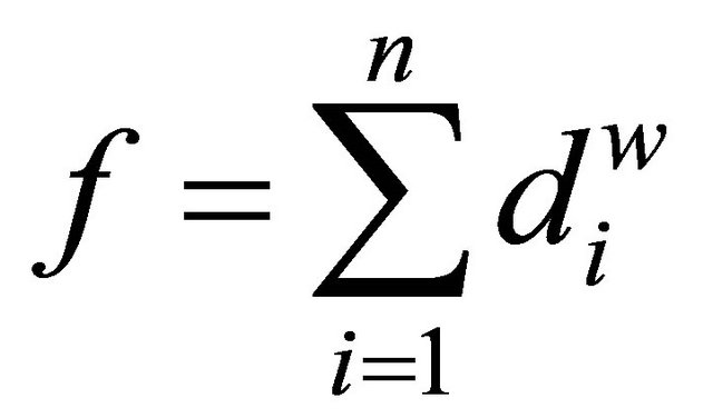 (1)
(1)
where the residual  represents the minimum distance between the i-th point of
  and its corresponding point on F and
  indicates the order of the residual. Then
  is given by:
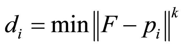 (2)
(2)
where  is the norm-degree to calculate the distance.
To minimize  and find the best surface fit, some variables are tunned. These variables are specific for each situation. Table 1 shows the decision variables for each surface addressed in this paper. On the other hand, norm
  remains constant in the optimization process and is considered as a parameter of the problem.
Table 1. Decision variables in analytic surfaces fitting.
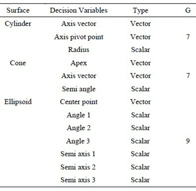
The number of decision variables  and the number of equality constrains
  in a optimization problem, allow to know the degrees of freedom with the equiation
 . Table 1 presents the degrees of freedom for each analytic surface addressed in this paper. Notice that
  corresponds to
  because the problem is unconstrained.
1.2. Optimization Method
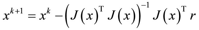
The Gauss-Newton iterative method for solving non-linear optimization problems uses the Hessian approximation 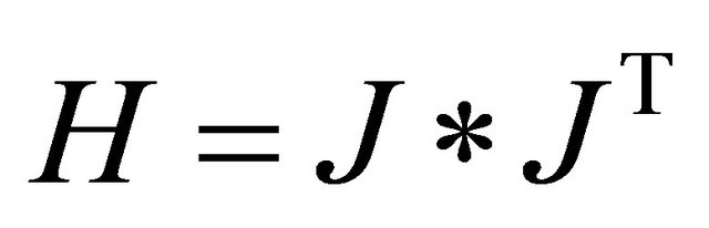 to calculate the next iteration, as is shown in Equation (3).
 (3)
(3)
where  is the decision variables vector and
  is residuals vector.
Notice that in the case in which  is not strictly convex,
  can be singular at some iteration possibly causing the algorithm to diverge. This problem can be overcome by using the Levenberg-Marquardt (LM) Method ([4,5]):
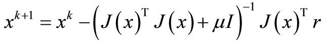 (4)
(4)
where  is the LM parameter and
  is the identity matrix.
1.3. Function and Region Convexity
The convexity condition of an objective function and its feasible region determines if a local extrema corresponds to a global extrema or not. In order to evaluate this condition in , it is required to examine the eigenvalues
  of its Hessian matrix
  by solving Equation (5)
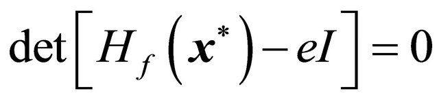 (5)
(5)
If all eigenvalues of  are positive, then
  is strictly-convex, but if at least one eigenvalue is equal to zero,
  is convex [6]. In the case studies on this research, an exact calculation of
  is not possible. Thus, a numerical calculation is required by approximating partial derivatives numerically.
2. Literature Review
2.1. Objective Function and Distance Measurement
Some authors have researched the calculation of the distance between a point and an analytic surface. Sappa and Rouhani [7] present a new technique for the estimation a pseudo geometric distance by calculating the height of a small tetrahedron intersecting the surface. This technique is prone to yield accuracy loss in the distance metric when applied to surfaces with high curvatures. Wang and Yu [1] present a comparison of the fitting processes implementing the algebraic, Euclidean, tangent or squared distance for fitting quadric surfaces. Zhou and Salvado [8] compare the geometric and algebraic distances in fitting ellipsoids. The authors estimate the geometric distance as the difference between the length of the ray connecting the point to ellipsoid center and the radius in the intersection of the ray and the surface. This estimation being a fast solution, only works well in cases of quasi-spherical ellipsoids.
2.2. Optimality Conditions
Just like Zhou and Salvado [8], Jiang and Cheng [9] classify the surface fitting problem as a non-convex one. The authors do not discuss the convexity analysis neither for the objective function nor for the optimization region. Other references reviewed do not report any classification of the surface fitting problem in terms of the convexity.
2.3. Optimization Methods
Yan, Liu and Wang [10] use Lloyd iterations to reconstruct quadric surfaces from a 3D point cloud. Ying, Yang and Zha [11] fit ellipsoids to data using semidefinite programming obtaining low runtime.
Jiang and Cheng [9] apply a decomposition technique to reduce the dimensions of the optimization space. This implies that the possibilities of dropping into local minima decrease. However, as the approach is out of the geometrical field, coming up with an initial guess of the parameters is not an easy task.
Li and Griffiths [12] fit ellipsoids by a least squares method using quadrics. This method does not require an initial estimation but, as it is not based on real geometrical distances, the results do not provide the best geometric fitting ellipsoid.
References [8,13] report the use of LM method to fit analytic surfaces without mentioning the selection of the LM parameter and its influence on the optimization process.
2.4. Initial Guess
Numerical optimization strategies are sensitive to the initial guess. The closer to the ideal solution is the initial guess, the less number of iterations in the optimization process. On the other hand, a bad initial guess could make the algorithm to diverge.
Just like Ruiz and Cadavid [14], Kwon et al. [15] use PCA for finding an approximation to axis orientation, center coordinates and radius of point clouds belonging to circular cylindrical surfaces. Because this technique reduces the dimensionality of the data giving the direction of largest dispersion [16], it is limited to cylinders with aspect ratio lower than 5.0 [14] and to cylindrical caps. Similarly, Zhou and Salvado [8] use the eigenvectors of the covariance matrix of the whole data as the axes of the ellipsoid coordinate system. As noted, this technique gives axes that probably will not correspond to the ellipsoid coordinate system in the case of ellipsoidal caps.
Simari and Singh [17] estimate the ellipsoid’s center as the geometric centroid of the data set. This proposal works in the cases of ellipsoids completely sampled but it loses validity when the cloud is only a subsample of the whole ellipsoid.
References [13,18] report the implementation of an algebraic method based on a least squares solution of the general quadric equation to find an initial guess of the parameters of analytic surfaces.
2.5. Literature Review Conclusions and Contribution of This Paper
As was shown in the taxonomy conducted in the literature review, there are several issues that remain open in optimized analytic surfaces fitting which are studied in this work: 1) Estimation of the real geometric distance between a point and an ellipsoid, 2) Identification of the effect of the parameters such as the norm k in the distance measurement, 3) Analysis of the optimality conditions effect on the convergence of the algorithm.
3. Methodology
3.1. Circular Cylinder Fitting
A circular cylinder is defined by a radius , an axis vector and its pivot point
  and
and  respectively. For purposes of this research, no assumption is made on the orientation or position in space of the cylinder from which the data set belongs.
3.1.1. Initial Guess for Circular Cylinder
The initial guess of the cylinder’s parameters is obtained with a statistical and geometrical procedure as explained below and shown in Figure 1:
1) Random seed points are selected from  and a local neighborhood
  found for each seed. See Figure 1(a).
2) Crossing each other the line segments defined by a seed point and the normal vector  of the best plane fit to
 , a set of points
  passing near
  are found. See Figure 1(b).
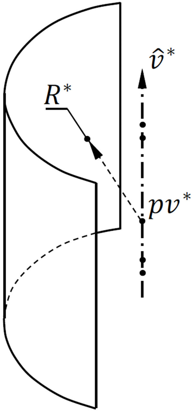
3) A PCA is executed over  for finding an initial approximation of the cylinder axis and its pivot point,
  and
and  respectively. See Figure 1(c).
4) An approximation to the cylinder radius is calculated as the average of the minimum distances between  and
and .
.
This method allows processing both complete cylindrical surfaces and cylindrical caps.
3.1.2. Estimation of Point-Cylinder Distance
The minimum distance  between the point
  and a circular cylindrical surface is calculated as:
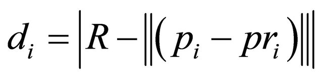 (6)
(6)
where  is the radius of the cylinder and
  is the orthogonal projection of
  onto
onto  as is shown in Figure 2.
3.2. Circular Cone Fitting
A circular right cone can be defined by an axis vector , an apex
  and a semi-opening angle
 .
.
3.2.1. Initial Guess for Circular Cone
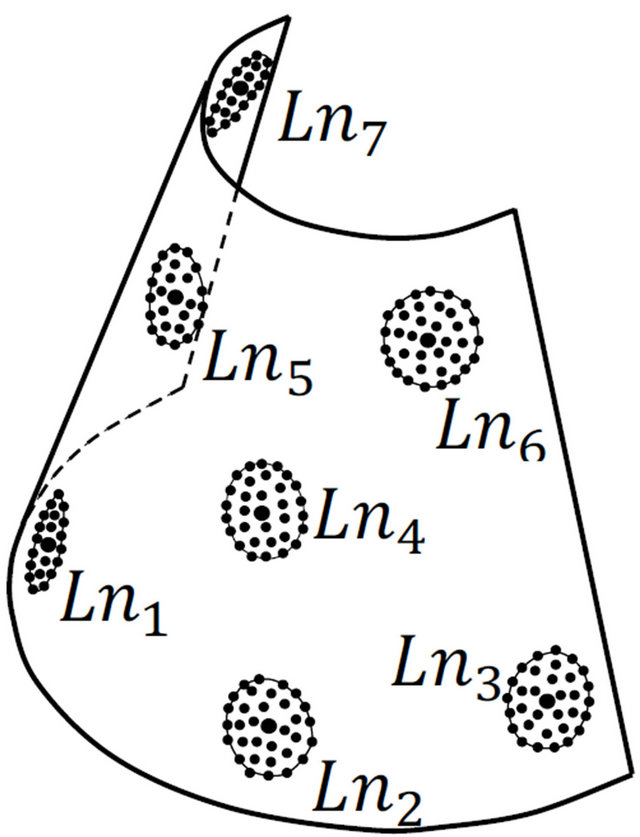
The initial approximation of a circular conical surface to a point cloud is obtained by an statistical and geometrical procedure as is depicted in Figure 3 and explained as follows:
1) A set of seed points and local neighborhoods  are taken from
 . See Figure 4(a).
2) The minimum curvature direction  of
of ,
,
 (a)
(a)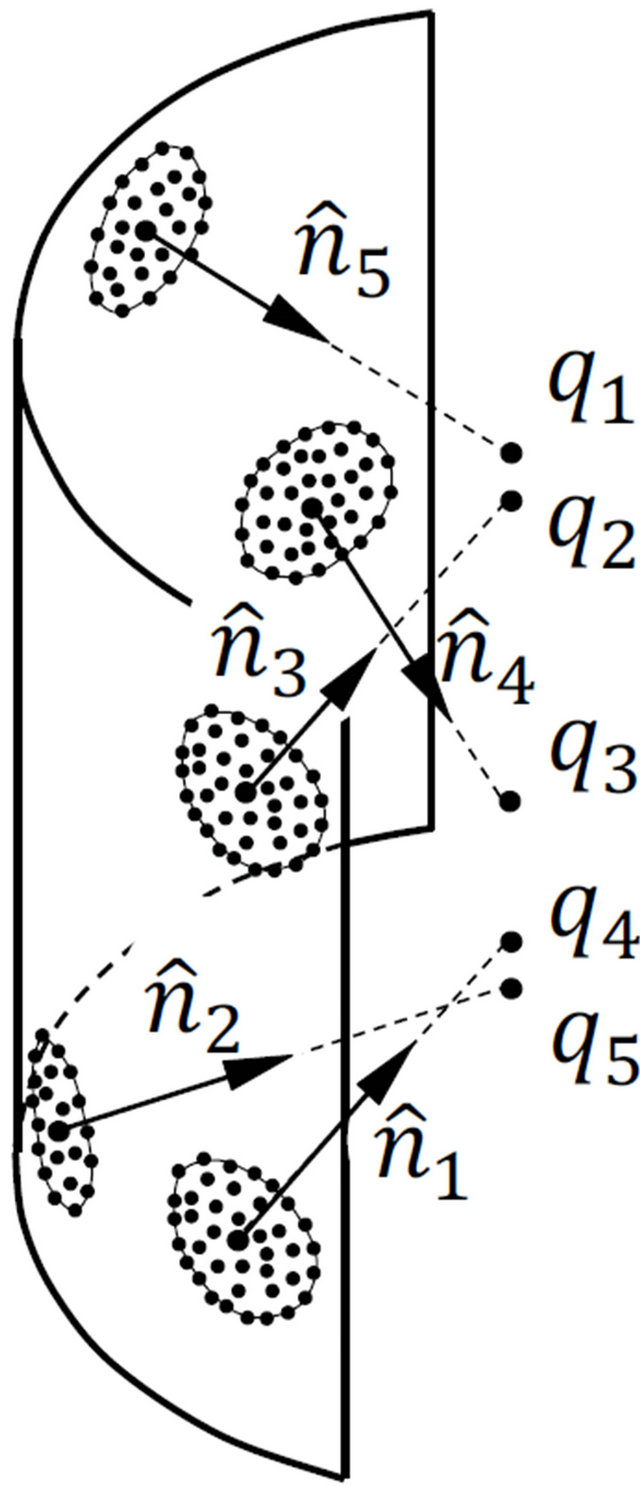 (b)
(b)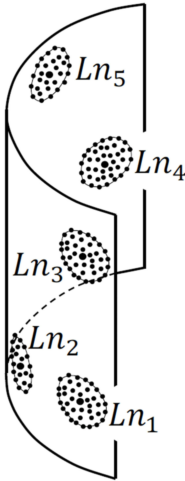 (c)
(c)
Figure 1. Initial estimation of cylinder parameters. (a) Seed points and the local neighborhoods; (b) Crossing line segments defined by the normal vector of the best planet to Ln; (c) Statistical axis and radius of the cylinder.
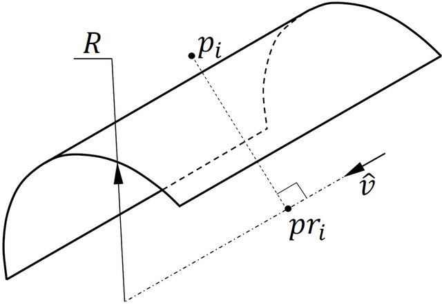
Figure 2. Calculation of point-cylinder distance.
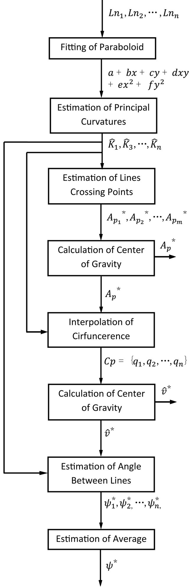
Figure 3. Procedure for obtaining the initial guess of conical sample.
being collinear with a generatrix of the cone, is found by fitting a paraboloid  and calculating the eigenvectors of it Hessian matrix
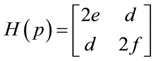 . See Figure 4(b).
3)  being the first approximation to
 , is obtained by averaging the crossing points of all lines defined by a seed point and its corresponding
 . Notice that
  represents an statistical apex. See Figure 4(c).
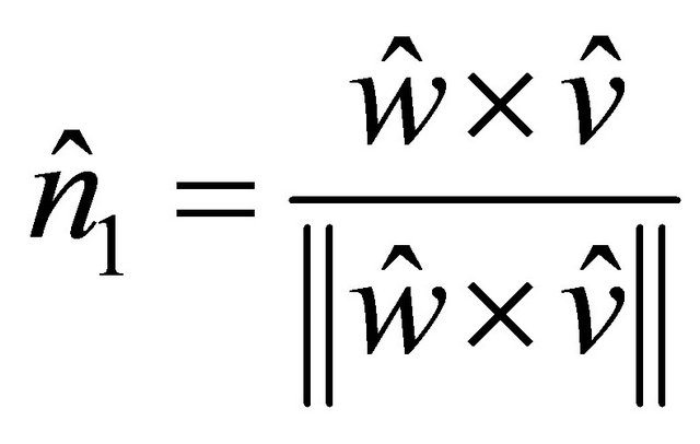
4) By finding the center of gravity of the center of the circumferences passing trough the points ,
,  and
and , where
  and
and  are unitary vectors in direction of minimum curvatures, the initial guess of the axis vector
  is
is
 (a)
(a)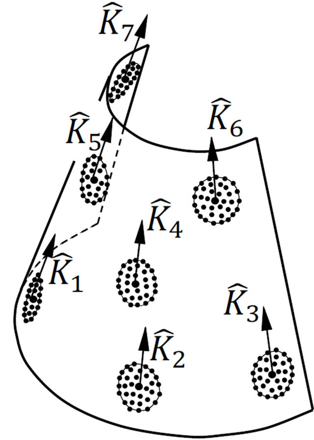 (b)
(b)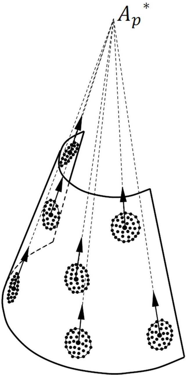 (c)
(c) (d)
(d)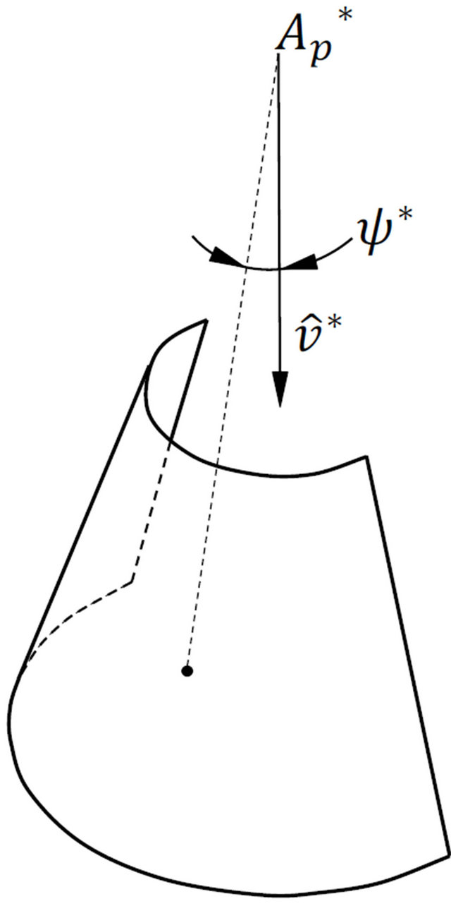 (e)
(e)
Figure 4. Initial estimation of cone parameters. (a) Seed points and them local neighborhoods; (b) Minimum curvarture directions; (c) Statistical apex point; (d) Statistical axis vector; (e) Statistical semi opening angle.
calculated. See Figure 4(d).
5) The initial estimation of  is taken as the average of the angles between the vectors
  and
and . See Figure 4(e).
3.2.2. Point-Cone Distance Estimation
The distance  from a point
  and a cone is calculated by solving the Equation (7) for
  and
and .
.
 (7)
(7)
where  is a rotation of
  around
  an angle
 ,
,
 and
and 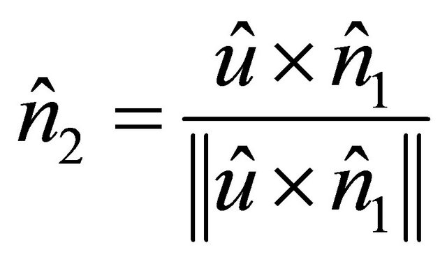 as is shown in the Figure 5. Finally
  is the signed distance between
  and the cone.
3.3. Ellipsoid Fitting
As is shown in Table 1, an ellipsoid in general position is defined by the center coordinates , the semi axes
  and the Euler angles
 .
.
3.3.1. Initial Guess for Ellipsoid
The first approximation to the parameters of the ellipsoid can be obtained with the following procedure:
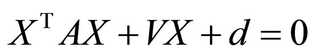
1) A general quadric surface is defined by Equation (8).
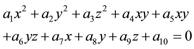 (8)
(8)
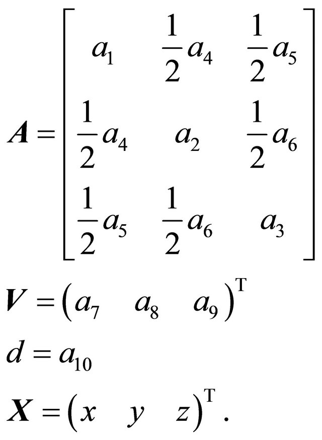
Rearranging Equation (8) appropriately [18], it can be written as:
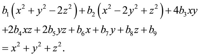
In compact form, the above equation is:
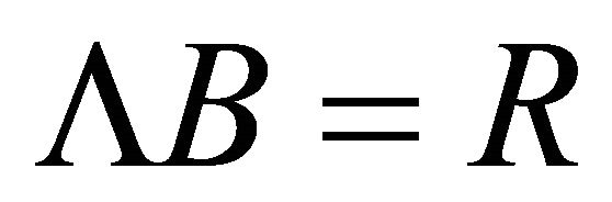 (9)
(9)
If the  points of
  are taken into account,
  is a
is a  matrix where its row
  -th is:

 is a
is a  vector with row
  -th:
-th: .
.  is the coefficients vector and it can be obtained by solving the linear system of Equation (9). As the system is overspecified, a least squares solution is calculated the with the pseudo-inverse matrix of
 :
:

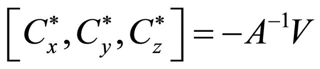
2) The initial approximation of the center coordinates , the semi axes
  and the Euler angles
 , are obtained from the subdiscriminant
  in the matrix notation of a general oriented quadric:
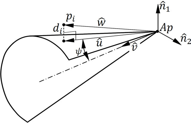
Figure 5. Calculation of point-cone distance.
 (10)
(10)
where
The eigenvectors of  represent the axes of the ellipsoid, then
  and
and  can be calculated. The eigenvalues of
  are proportional to
 and
and  [19], then
  and
and  can be obtained. The initial guess of the ellipsoid center can be obtained as
 .
.
3.3.2. Point-Ellipsoid Distance Estimation
We present the following conjecture (Figure 6).
Conjecture. Let  be an ellipsoid centered in
  i with Euler angles
  and semi axes
 . Let
. Let  be a point in
 . Then, an ellipsoid
  exists with the same center and orientation to
 , but with semi axes
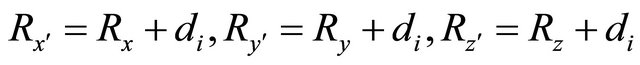 , that contain
 .
.
If  and
and  are translated to the origin and aligned with the principal axes by a rigid transformation, the following equation can be posed:
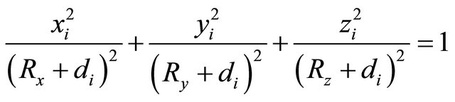 (11)
(11)
Rearranging (11):
 (12)
(12)
where 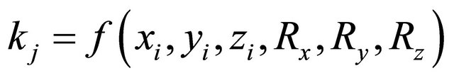 with
with .
.
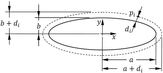
Figure 6. Calculation of point-ellipsoid distance.
The minimum absolute real root of the polynomial in Equation (12) corresponds to the minimum signed distance from  to
to .
.
4. Results and Discussion
In order to test our fitting routines two study cases were proposed as follows.
4.1. Data Set 1. Frog
In order to prove the algorithm for fitting ellipsoids, a subset of the frog shown in Figure 7(a) was taken. In Figure 7(b) the highlighted points to which the ellipsoids were fitted can be seen. The result of the fitting process is presented in Figures 7(c) and (d).
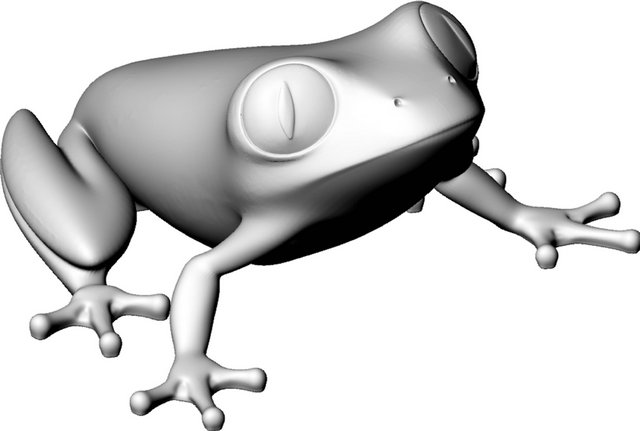
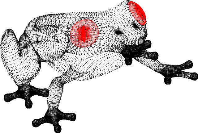
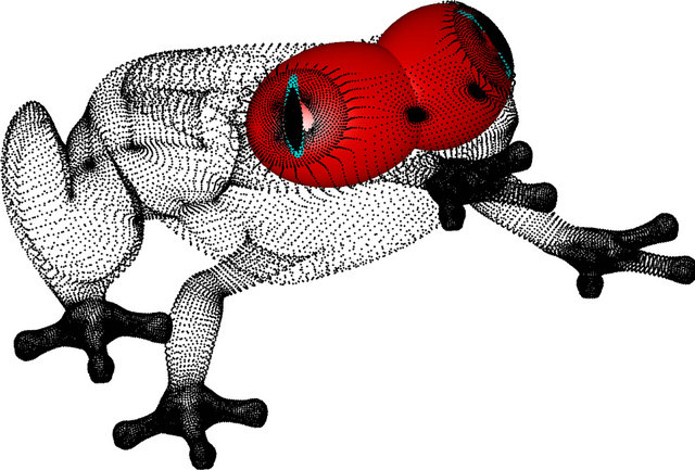
(a) Frog model (b) Frog point cloud (c) Ellipsoid fitting results. View 1 (d) Ellipsoid fitting results. View 2
Figure 7. Ellipsoid fitting results. Original 3D model obtained from Thingiverse® [20].
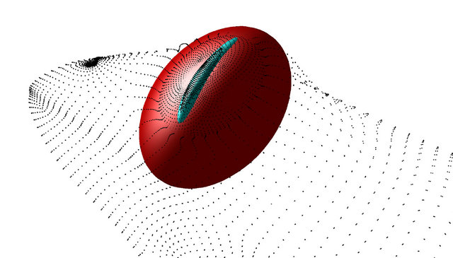
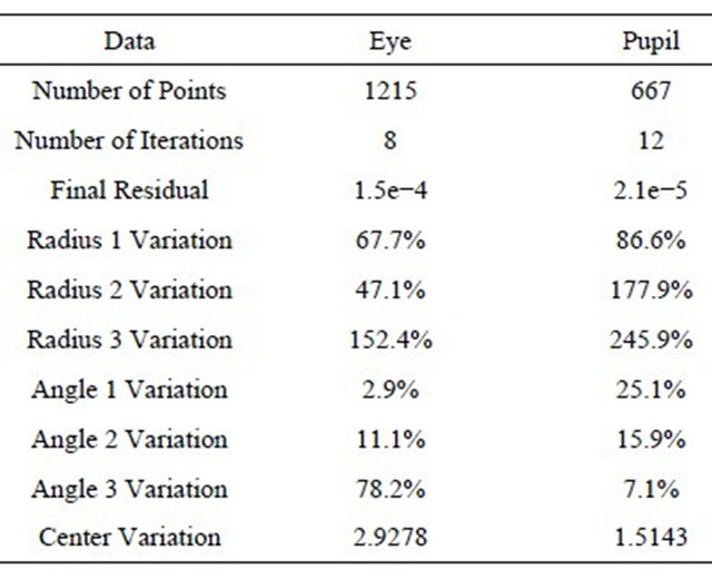
A good initial guess found by an algebraic approach, let to a fast convergence of the algorithm. In Figure 8 it may be seen that the longest fitting process required of 12 iterations for finding the optimum according to the termination criteria. In Figure 9 the initial estimation ellipsoid and the best geometrical ellipsoid fit are shown. Notice that the initial surface wraps most of the points, giving a good starting point for the LM algorithm. Table 2 presents a comparison between the the initial ellipsoids and the optimized ones.
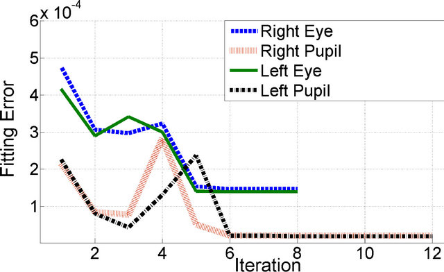
Figure 8. Behavior of objective function in the optimization process.

Figure 9. Comparison between initial guess and optimization results in ellipsoid fitting.
Table 2. Fitting results in frog’s study case.
4.2. Data Set 2. Fan
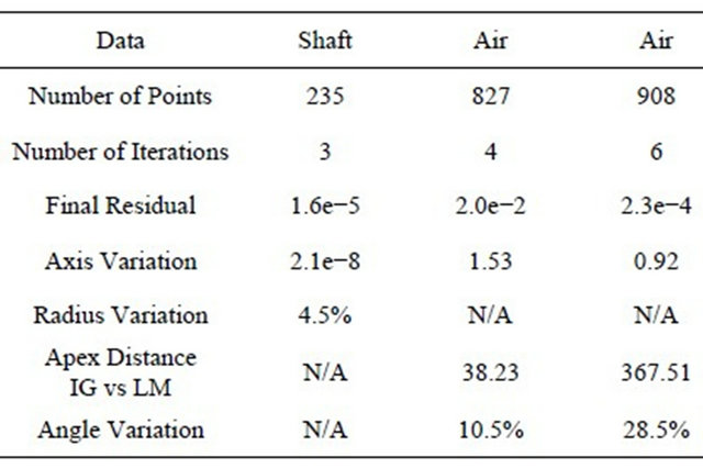
To test the cylinder and cone fitting algorithms some parts of the fan shown in Figure 10(a) were processed with the algorithms. Figure 10 displays the results of the optimization process of two conical surfaces and one cylinder. As in the case of ellipsoids, the algorithm found the optimal surface after a few iterations. The history of the optimized function for the Fan Data Set is shown in Figure 11. The cones (Figure 12) required 4 iterations while the cylinders (Figure 13) required 6 iterations. The good initial estimation of the surfaces allows the convergence of the algorithm and to reduce the number of iterations, therefore saving computing resources. Geometrical statistics for the Fan Data Set appear in Table 3.
Table 3. Fitting results in fan’s study case.

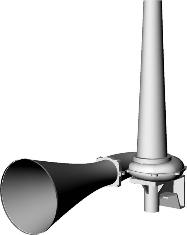
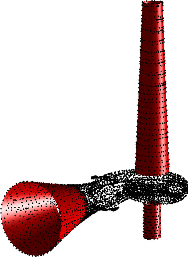
(a) Fan model (b) Fan point cloud (c) Cone and cylinder fitting results
Figure 10. Fan study case fitting results. Original 3D model obtained from GrabCAD® [21].
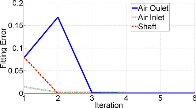
Figure 11. Behavior of objective function in the optimization process of the fan parts.
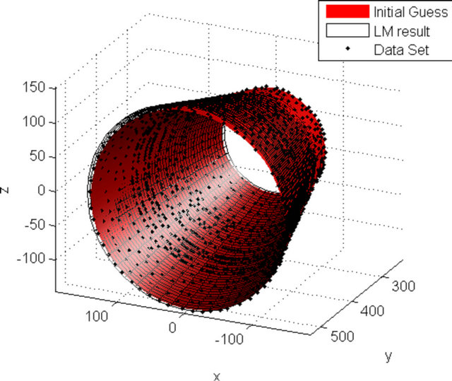
Figure 12. Comparison between initial guess and optimization results in cone fitting.
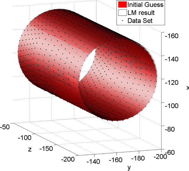
Figure 13. Comparison between initial guess and optimization results in cylinder fitting.
5. Conclusions and Future Work
This article presents the fitting of analytic surfaces (such as cylinders, cones and ellipsoids) in the sense of mathematical optimization. The objective function for each surface was implemented in terms of the real geometric distance. In the case of cylinder and conical surfaces this metric is formulated and calculated easily. However, in the ellipsoid case the measurement of the distance between a point and the surface is not trivial. In response to this situation this work presented a novel methodology to calculate this distance. The addressed results allow to check that the proposed distance calculation works fine.
The routines for the initial guess of the surfaces were implemented using geometrical and statistical procedures. The study cases allow to prove that the iterative optimization algorithms converge fast with a good initial guess.
Future work includes the extension of the optimization strategies to other analytic and to free form parametric surfaces.
REFERENCES
- H. Nyquist, “Certain Topics in Telegraph Transmission Theory,” Transactions of the American Institute of Electrical Engineers, Vol. 47, No. 2, 1928, pp. 617-644. doi:10.1109/T-AIEE.1928.5055024
- C. E. Shannon, “Communication in the Presence of Noise,” Proceedings of the IRE, Vol. 37, No. 1, 1949, pp. 10- 21. doi:10.1109/JRPROC.1949.232969
- K. Levenberg, “A Method for the Solution of Certain Non-Linear Problems in Least Squares,” Quarterly Journal of Applied Mathmatics, Vol. II, No. 2, 1944, pp. 164- 168.
- D. W. Marquardt, “An Algorithm for Least-Squares Estimation of Nonlinear Parameters,” Journal of the Society for Industrial and Applied Mathematics, Vol. 11, No. 2, 1963, pp. 431-441. doi:10.1137/0111030
- E. K. P. Chong and S. H. Zak, “An Introduction to Optimization,” 2nd Edition, Wiley India Pvt. Ltd., New Delhi, 2010.
- J. Wang and Z. Yu, “Quadratic Curve and Surface Fitting Via Squared Distance Minimization,” Computers and Graphics, Vol. 35, No. 6, 2011, pp. 1035-1050. doi:10.1016/j.cag.2011.09.001
- A. D. Sappa and M. Rouhani, “Efficient Distance Estimation for Fitting Implicit Quadric Surfaces,” 16th IEEE International Conference on Image Processing ICIP, Cairo, 7-12 November 2009, pp. 3521-3524.
- D. M. Yan, Y. Liu and W. Wang, “Quadric Surface Extraction by Variational Shape Approximation,” Geometric Modeling and Processing—GMP, Pittsburgh, 26-28 July 2006, pp. 73-86.
- X. Jiang and D. C. Cheng, “A Novel Parameter Decomposition Approach to Faithful Fitting of Quadric Surfaces,” Pattern Recognition, Vol. 3663, 2005, pp. 168- 175. doi:10.1007/11550518_21
- X. Ying, L. Yang and H. Zha, “A Fast Algorithm for Multidimensional Ellipsoid-Specific Fitting by Minimizing a New Defined Vector Norm of Residuals Using Semidefinite Programming,” IEEE Transactions on Pattern Analysis and Machine Intelligence, Vol.:1856--1863, 2012. doi:10.1109/TPAMI.2012.109
- Q. Li and J. G. Griffiths, “Least Squares Ellipsoid Specific Fitting,” Proceedings of Geometric Modeling and Processing, 2004, pp. 335-340. doi:10.1109/GMAP.2004.1290055
- S. W. Kwon, F. Bosche, C. Kim, C. T. Haas and K. A. Liapi, “Fitting Range Data to Primitives for Rapid Local 3D Modeling Using Sparse Range Point Clouds,” Automation in Construction, Vol. 13, No. 1, 2004, pp. 67-81. doi:10.1016/j.autcon.2003.08.007
- O. Ruiz and C. Vanegas, “Statistical Assessment of Global and Local Cylinder Wear,” 5th IEEE International Conference on Industrial Informatics, Vienna, 23-26 July 2007, pp. 387-392.
- R. A. Calvo, M. Partridge and M. Jabri, “A Comparative Study of Principal Component Analysis Techniques,” Proceedings of Ninth Australian Conference on Neural Networks, Brisbane, 11-13 February 1998, pp. 276-281.
- L. Zhou and O. Salvado, “A Comparison Study of Ellipsoid Fitting for Pose Normalization of Hippocampal Shapes,” International Conference on Digital Image Computing Techniques and Applications (DICTA), Noosa, 6-8 December 2011. pp. 285-290.
- P. D. Simari and K. Singh, “Extraction and Remeshing of Ellipsoidal Representations from Mesh Data,” Proceedings of Graphics Interface, 9-11 May 2005, Canadian Human-Computer Communications Society, pp. 161-168.
- D. Marshall, G. Lukacs and R. Martin, “Robust Segmentation of Primitives from Range Data in the Presence of Geometric Degeneracy,” IEEE Transactions on Pattern Analysis and Machine Intelligence, Vol. 23, No. 3, 2001, pp. 304-314. doi:10.1109/34.910883
- D. A. Turner, I. J. Anderson, J. C. Mason and M. G. Cox, “An Algorithm for Fitting an Ellipsoid to Data,” National Physical Laboratory, Teddington, 1999.
- J. Wallner, “On the Semiaxes of Touching Quadrics,” Resultate der Mathematik, Vol. 36, No. 3-4, 1999, pp. 373- 383. doi:10.1007/BF03322124
- P. Morena at Thingiverse, “Treefrog STL Model,” 2012. http://www.thingiverse.com/download:61236
- E. Carlos at GrabCAD, “Fan STL Model,” 2012. http://grabcad.com/library/carcasa-de-un-ventilador-para-ensayos/files/carca.stl
Nomenclature
S:  Noisy point sample F: Best fit surface to S PCA: Principal Component Analysis LM: Lenvenberg-Marquardt k: Norm degree f: Objective function di: Minimum distance between the i-th point of
  and its corresponding point on F