American Journal of Computational Mathematics
Vol.2 No.3(2012), Article ID:23180,8 pages DOI:10.4236/ajcm.2012.23025
Some Examples to Show That Objects Be Presented by Mathematical Equations
Department of Mathematics and Statistics, Bowling Green State University, Bowling Green, USA
Email: tmtran@bgsu.edu
Received March 30, 2012; revised June 16, 2012; accepted june 24, 2012
Keywords: Graph, Equation; Visible and Invisible Object
ABSTRACT
We have often heard remarks such as “We can plot graphs from the mathematical equations”, including equations of lines, equations of curves, and equations of invisible and visible objects. Actually, we can present each object by mathematical equation and we can plot graphs from equations. Equations not only show visible objects but also can show invisible objects such as wave equations in differential equations. In fact, the change of equations is also to conduce the change of objects and phenomena. This paper presents mathematical equations, methods to plot the graphs in 2D and 3D space. The paper is also a small proof of this conclusion have been provided and addressing visualization problem for any object. The novelty of this paper presents some special equations of objects and shows the ideas to build objects from equations.
1. Introduction
In this section, we will briefly review some basic and special equations in 2D and 3D space. In 2D space, we will plot graphs of simple linear equations, equation of circles, and some special equations as equation of heart in Cartesian coordinates and Polar coordinate to show the attitude of objects. In 3D space, we have a change from equations in two variables in 2D space to equations in three variables in 3D space. We use some special functions in Mathematica to plot graph of objects, including sphere, hearts, apple, and wave equations. In addition, we can plot an object in two different coordinate systems to present mathematical methods and functions in Mathematica.
1.1. In 2D Space
1.1.1. In Cartesian Coordinates
We can plot linear equation as follows:
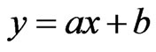
The graph of this equation is a line.
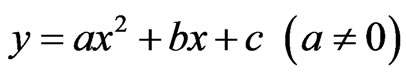
We also plot the graph of higher order equations such as Quadratic equation:
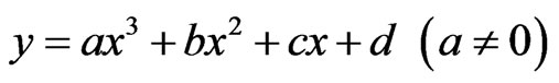
Cubic equation:
And higher order equations. Graph of these equations are curves.
1.1.2. In Polar Coordinate
We can plot some graphs in this coordinate. We will use two variables in the equation.
Generally, we will introduce the equation of circles with the form:

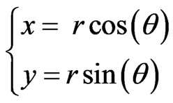
We will vary from Cartesian coordinate to Polar coordinate by using form:
1.2. In 3D Space
In this section, we will plot equations in two coordinate systems and will show equation of sphere in the two mathematical methods
1.2.1. In Cartesian Coordinates
We will plot some objects in 3D space to see a relationship between equations and graphs. We will use equation in three variables.
Generally, we rewrite equation of sphere with the following form:
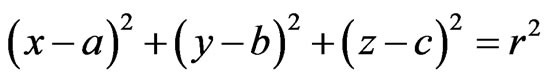 where
where  is center of the sphere.
1.2.2. In Polar Coordinate
We can vary equation of sphere to polar coordinates as follows :

where :
:
2. Some Equations in Cartesian Coordinates
2.1. Linear Equation
We see that linear quation with the following form:
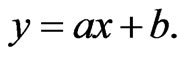
With a = 0, we have the equation y = b, with b = 2 or b = −2.
Using Mathematica software to plot these graphs In Mathematica
Input: Plot 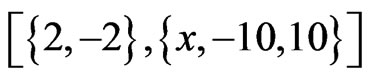
Press “Shift-Enter”} at the end of the command line. See Figure 1.
We have the graphs of the equations:
Where a > 0, we will plot the equation y = 2x.
Input: Plot 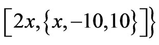
Press “Shift-Enter”} at the end of the command line. See Figure 2.
Where a < 0, we will plot the equation y = −2x.
Input: Plot 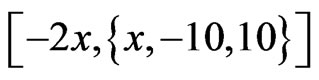
Press “Shift-Enter”} at the end of the command line. See Figure 3.
2.2. Quadratic Equation
We know that the graph of the quadratic equation has the form:

In Mathematica Where a > 0, we can plot the equation
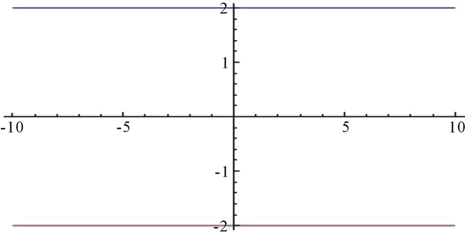
Figure 1. The graphs of the equations y = 2 and y = −2.
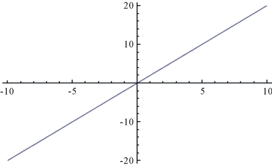
Figure 2. The graph of the equation y = 2x.
Figure 3. The graph of the equation y = −2x.
 .
.
Input: Plot 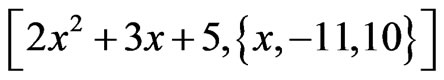
Press “Shift-Enter”} at the end of the command line. See Figure 4.
Where a < 0, we can plot the equation 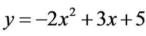 .
.
Input: Plot 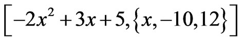
Press “Shift-Enter”} at the end of the command line. See Figure 5.
2.3. Cubic Equation
We know that the graph of the cubic equation:
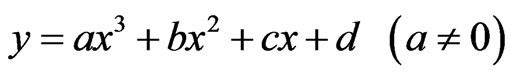
is a curve.
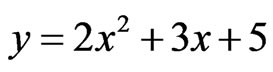
In Mathematica Where a > 0, we can plot the equation 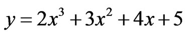 .
.
Input: Plot 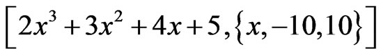
Press “Shift-Enter”} at the end of the command line. See Figure 6.
Where a < 0, we have the graph of 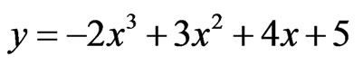 .
.
Input: Plot 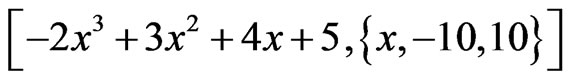
Press “Shift-Enter”} at the end of the command line. See Figure 7.
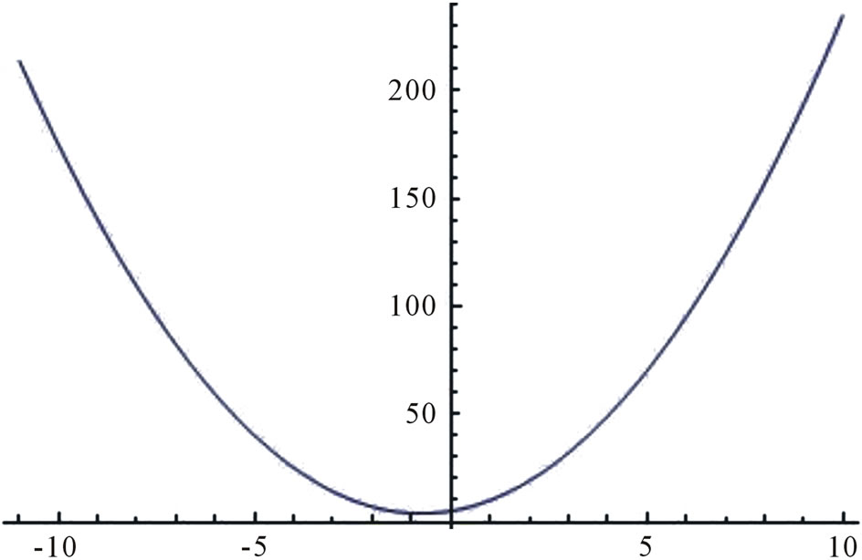
Figure 4. The graph of the equation y = 2x2 + 3x + 5.
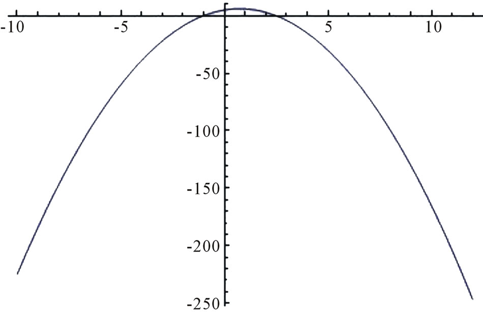
Figure 5. The graph of the equation y = −2x2 + 3x + 5.
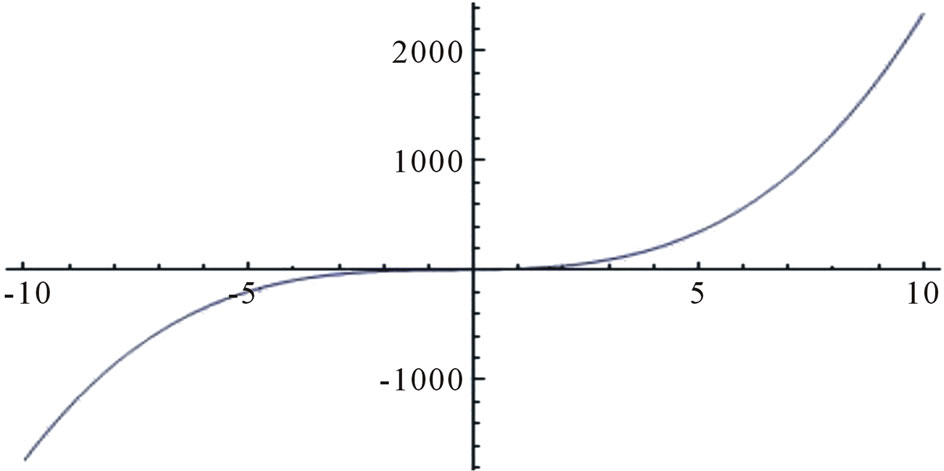
Figure 6. The graph of the equation y = 2x3 + 3x2 + 4x + 5.
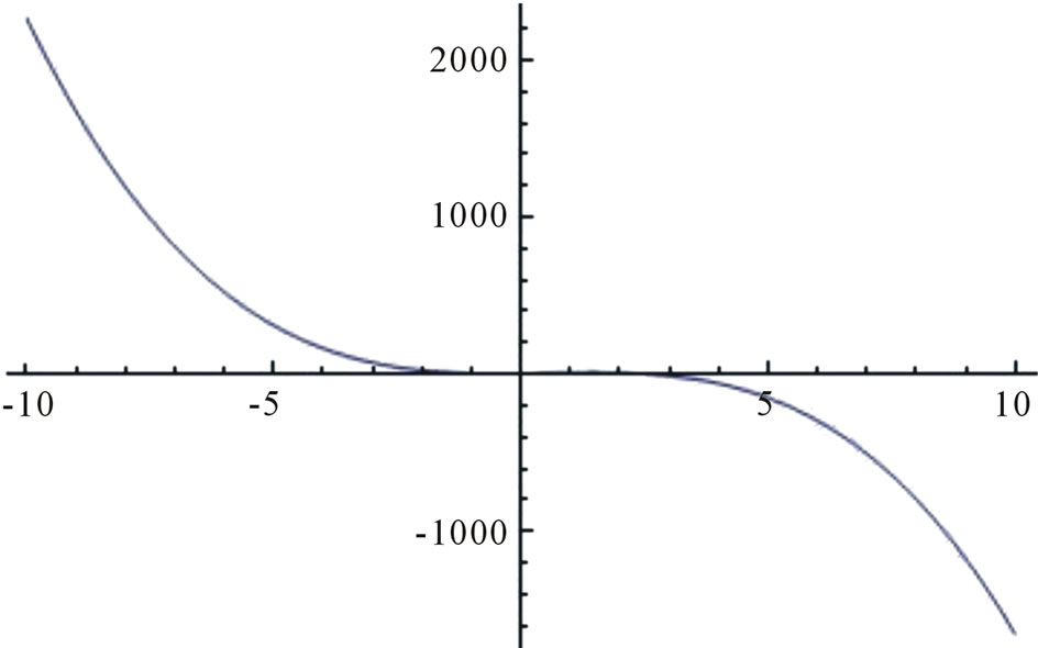
Figure 7. The graph of the equation y = −2x3 + 3x2 + 4x + 5.
2.4. Some Higher Order Equations
Quartic equation [1]
Plot graph of the equation:
Input: Plot 
Press “Shift-Enter”} at the end of the command line. See Figure 8.
Quintic equation

To plot graph of the equation:
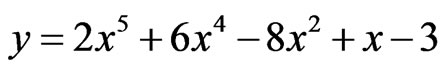
Input: Plot 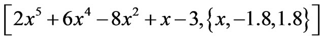
Press “Shift-Enter”} at the end of the command line. See Figure 9.
Plot graph of the equation:
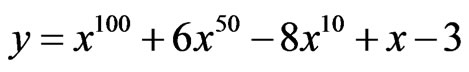
Input: Plot 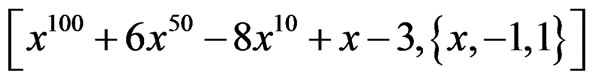
Press “Shift-Enter”} at the end of the command line. See Figure 10.
3. Some Equation in Polar Coordinates
3.1. Circle Equations
Generally, we will introduce the equation of circles
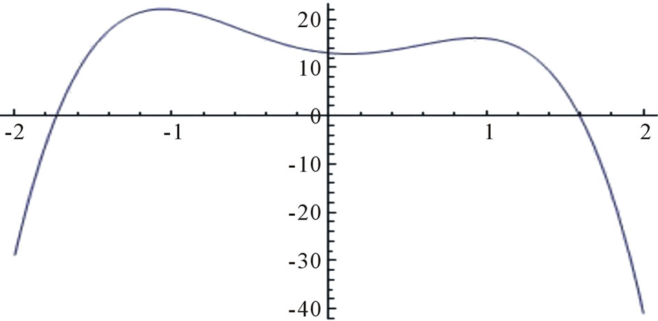
Figure 8. The graph of y = −6x4 + 12x3 + cx2 − 3x + 13 [1].
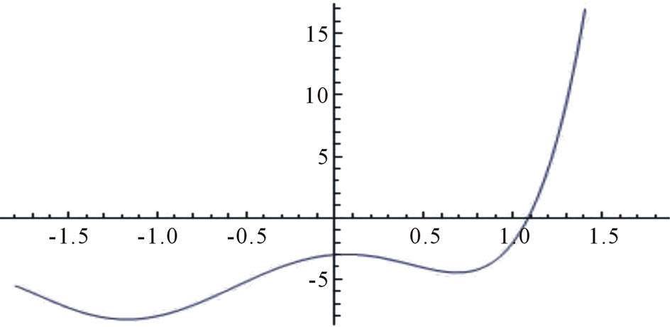
Figure 9. The graph of y = 2x5 + 6x4 − 8x2 + x − 3 100th order equation [2].
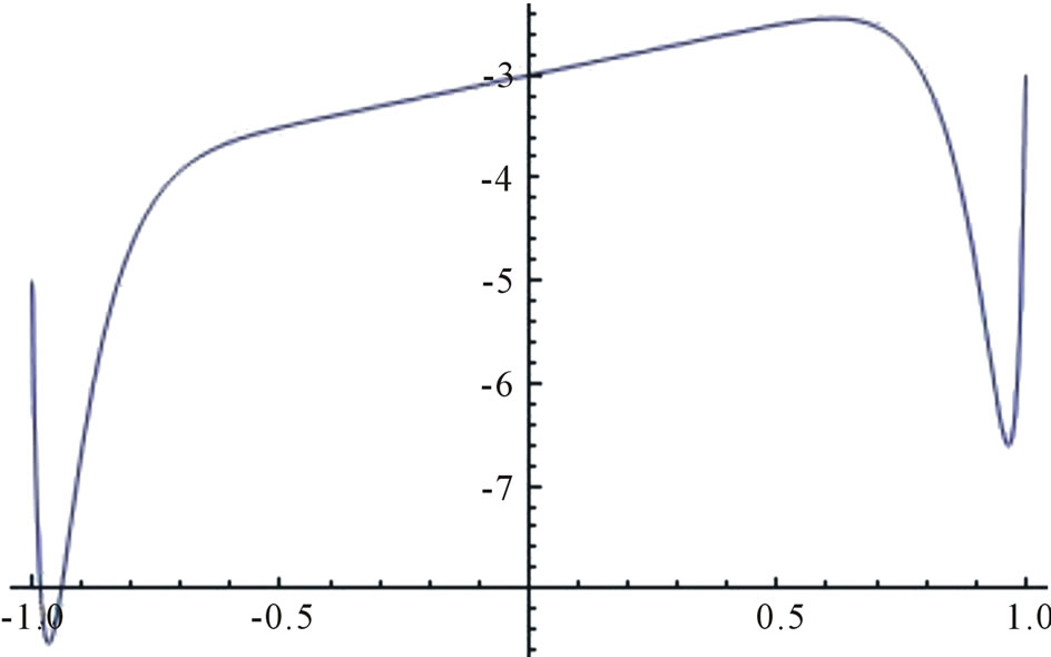
Figure 10. The graph of y = x100 + 6x50 − 8x10 + x − 3.
as follows:
Choose r = 2, a = b = 0. We have the equation 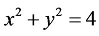
We can directly plot with the command.
Input: ContourPlot
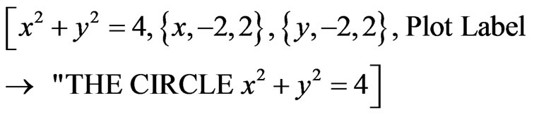
Press “Shift-Enter” at the end of the command line. See Figure 11.
We can vary to polar coordinates, where :
:
Set:
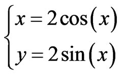
Plot graph of the equation in Mathematica.
Input: ParametricPlot
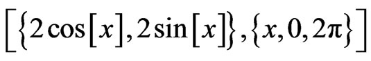
Press “Shift-Enter”} at the end of the command line. See Figure 12.
3.2. Elliptic Equations
In this section, we will plot the equations of three circles x = 3cost, y = 3sint; x = 2cost, y = 2sint; x = cost, y = sint and the equation of two elliptics:

Input: ParametricPlot
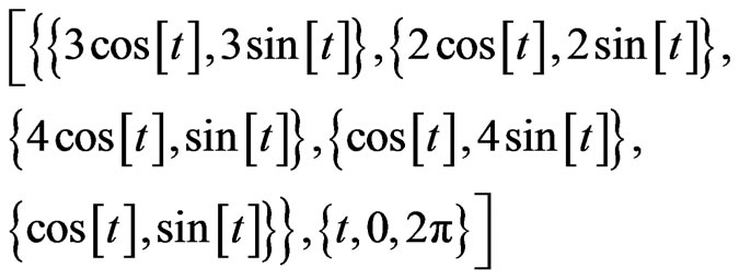
Press “Shift-Enter”} at the end of the command line. See Figure 13.
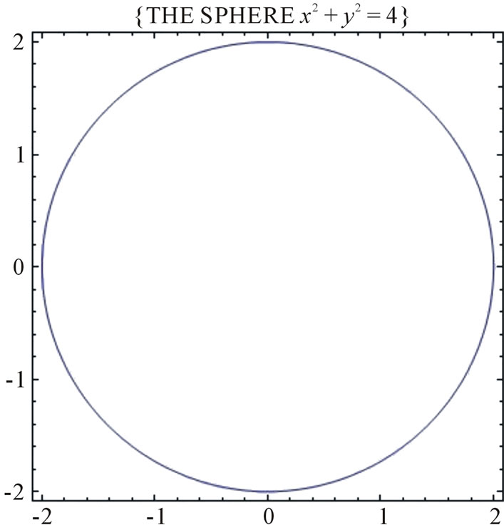
Figure 11. The graph of the circle in Cartesian coordinates.
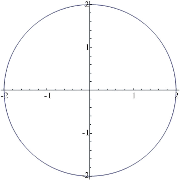
Figure 12. The graph of the circle in polar coordinates.
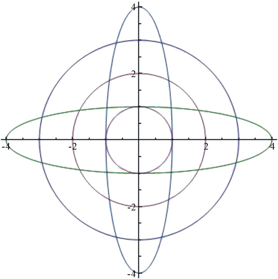
Figure 13. The graph of the elliptic equations.
3.3. The Equations of Heart [3]
From the general form, where :
:
We can revise the equation system to plot graph of heart
where .
.
Input: ParametricPlot
Press “Shift-Enter” at the end of the command line. See Figure 14.
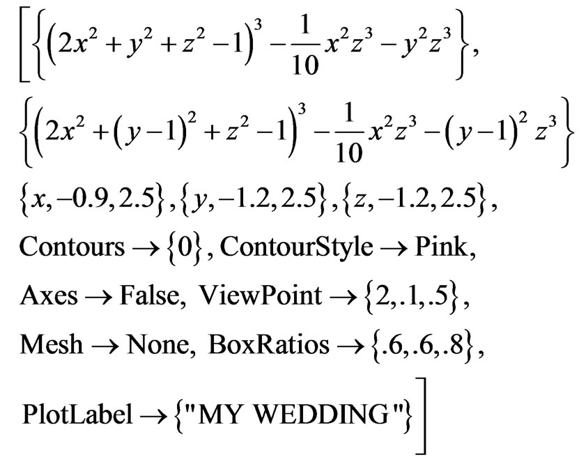
3.4. The Equation of Wedding [4]
From Eugen Beutel equation :
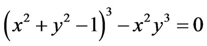
We will create a new equation in a command line to build two intersectional hearts in the graph.
We can set a name of the equation with title: “Song Hy Equation”.
Input: ContourPlot
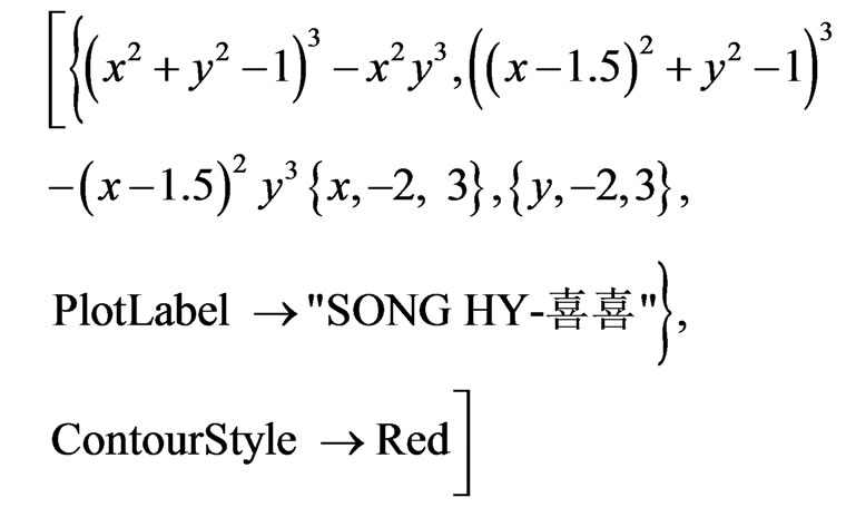
Press “Shift-Enter”} at the end of the command line. See Figure 15.
4. Some Equations in 3D Space
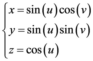
4.1. The Equation of Sphere
Generally, we will write the equation of sphere with form
 , where
 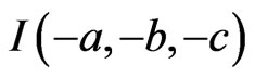 is centre of the sphere.
Choose r = 2, a = b = c = 0. We have the equation: 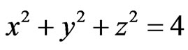

Figure 14. The graph of the heart.
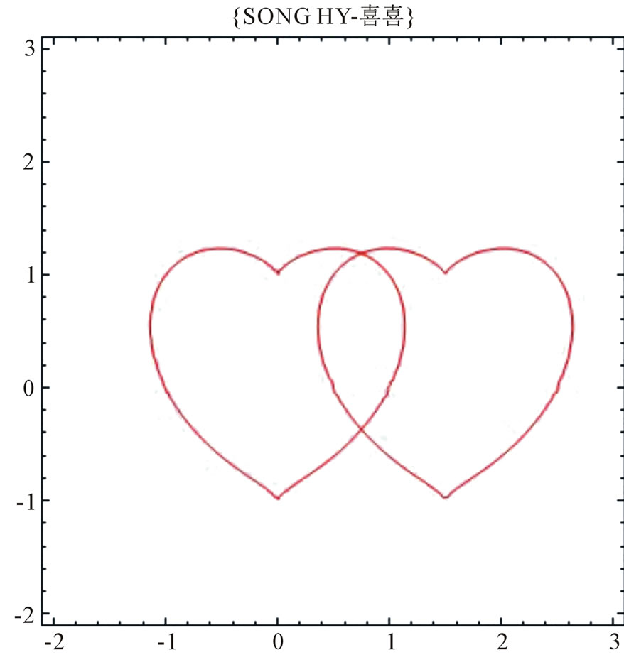
Figure 15. The graph of wedding (SONG HY-喜喜).
We can directly plot with the command.
Input: ContourPlot3D
Press “Shift-Enter” at the end of the command line. See Figure 16.
We can vary to polar coordinates, where :
:

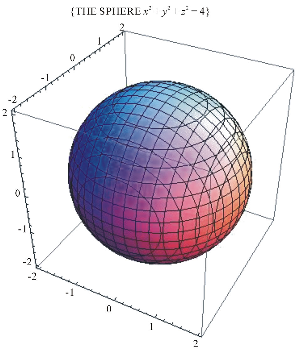
Figure 16. The graph of sphere in Cartesian coordinates.
Plot graph of the equation in Mathematica.
Input: ParametricPlot3D
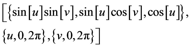
Press “Shift-Enter” at the end of the command line. See Figure 17.
4.2. The Equation of Apple
From the equation of sphere in polar coordinates as follows:
where 
We will vary the coordinates of x and y to create new coordinates system in 3D space.
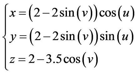
where .
.
The change of the equation shows that a new object has been created. The graph of new equation can be observed in the figure below. It is the same an apple and is called with title: “The equation of Apple”.
Input: ParametricPlot3D
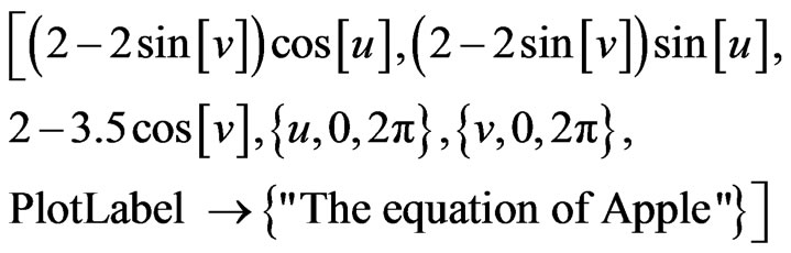
Press “Shift-Enter” at the end of the command line. See Figure 18.
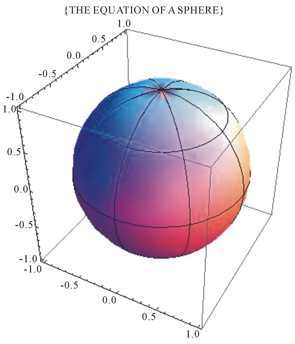
Figure 17. The graph of sphere in polar coordinates.
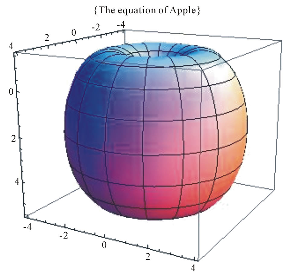
Figure 18. The graph of apple.
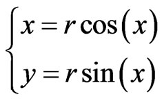
4.3. The Equation of Donuts Cakes [3]
According to Polar coordinates in 3D space, we can be plotted an object. By the change of the coordinates of equations, we can built the different attitude of objects From the combine of equations, we have plotted the rings in different colors in 3D space. These figures have called with title: “Donuts cakes”.
Input: ParametricPlot3D
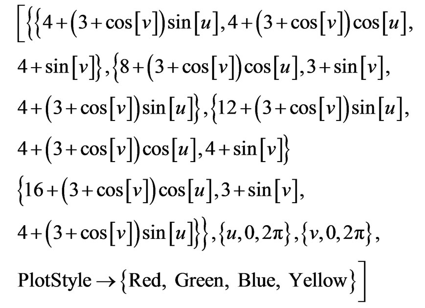
Press “Shift-Enter” at the end of the command line. See Figure 19.
4.4. The Wedding Equation [4]
From Gabriel Taubin equation:
We can vary and combine two equations in a command line to build a new object with the figure of two intersectional hearts.
We can set a name of this equation with title: “Wedding Equation”.
Input: ContourPlot3D
Press “Shift-Enter” at the end of the command line. See Figure 20.
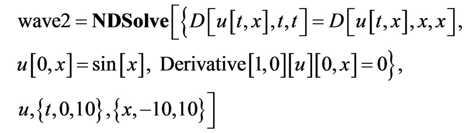
4.5. The Wave Equation in Plane [3]
We have the following differential equation:
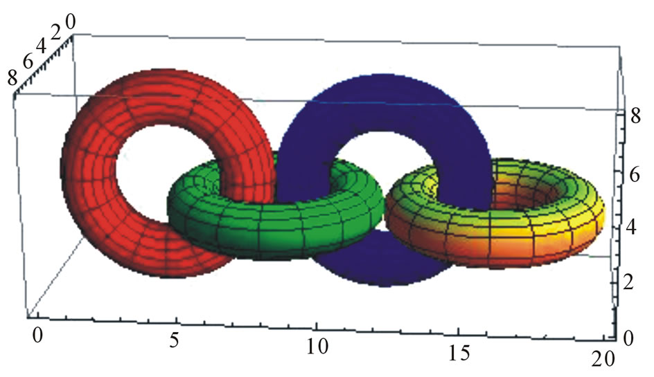
Figure 19. The graph of donuts cakes.
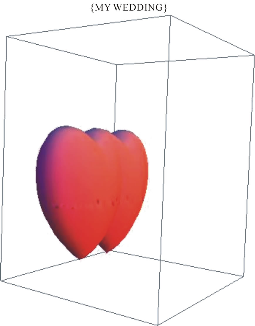
Figure 20. The graph of the wedding in space.
 , with initial condition
 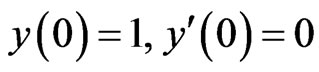 .
.
Using Mathematica software to plot the wave form of the equation as follows:
Input:
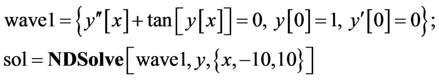
Input: Plot 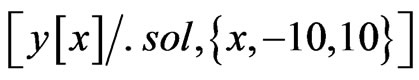
Press “Shift-Enter” at the end of the command line. See Figure 21.
4.6. The Wave Equation in Space [3]
We have the differential equation [5]
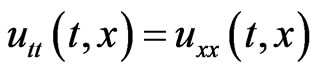 with initial boundary condition
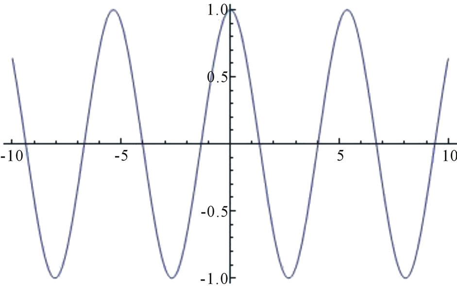
Figure 21. The graph of the wave equation in plane.
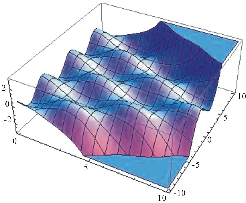
Figure 22. The graph of the wave equation in space.
 ,
, .
.
Using Mathematica to plot the wave form of this equation.
Input:
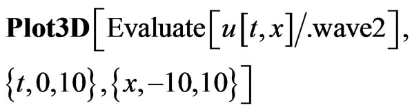
Press “Shift-Enter” at the end of the command line. See Figure 22.
5. Conclusions
This paper has shown some visible and invisible figures of the equations. In the paper, we have also discussed the equations and have presented the graphs of mathematical equations in 2D and 3D space. Each change of an equation is shown the change of object, so we will have a stronger understanding in relationship between equations and objects.
Indeed, we can plot any graphs from equations; contradictorily, from the objects are known, we can also find equations of these objects and how we can find these equations. I think, that is the future of work, which we can do to determine equations by softwares, mathematical modeling.
This paper also kindles new ideas about the change of equation. The use of Mathematica in this paper illustrates the important role of technology in research in mathematical equations. It not only help in providing a computing platform but also serves as a useful tool for plotting visual images resulting from the equation.
REFERENCES
- The Knowledge in Mathematica 7.0 Softwave,Wolfram as Gabriel Taubin Equation, and Others.
- The Minh Tran, “Using Scientific Calculators to Solve the Mathemtical Problems for Excellent Students,” Calculator Company, 2009.
- R. J. Lopez, “Advanced Engineering Mathematics,” Addison Wesley, Boston, 2000.
- R. T. Smith and R. Minton, “Calculus,” 3rd Edition, McGraw-Hill Companies, Inc., New York, 2011.
- http://www.mathematische-basteleien.de/heart.htm