American Journal of Computational Mathematics
Vol. 1 No. 1 (2011) , Article ID: 4450 , 4 pages DOI:10.4236/ajcm.2011.11004
A Third-Order Scheme for Numerical Fluxes to Guarantee Non-Negative Coefficients for Advection-Diffusion Equations
Saitama Institute of Technology, Fukaya, Japan
E-mail: sakai@sit.ac.jp, dw@sit.ac.jp
Received February 18, 2011; March 7, 2011; March 16, 2011
Keywords: Numerical Scheme, Numerical Analysis, Numerical Stability, Positivity Condition, Advection-Diffusion Equation, Advection Equation, High-Order Scheme, Godunov Theorem, Burgers’ Equation
Abstract
According to Godunov theorem for numerical calculations of advection equations, there exist no higher-order schemes with constant positive difference coefficients in a family of polynomial schemes with an accuracy exceeding the first-order. In case of advection-diffusion equations, so far there have been not found stable schemes with positive difference coefficients in a family of numerical schemes exceeding the second-order accuracy. We propose a third-order computational scheme for numerical fluxes to guarantee the non-negative difference coefficients of resulting finite difference equations for advection-diffusion equations. The present scheme is optimized so as to minimize truncation errors for the numerical fluxes while fulfilling the positivity condition of the difference coefficients which are variable depending on the local Courant number and diffusion number. The feature of the present optimized scheme consists in keeping the third-order accuracy anywhere without any numerical flux limiter by using the same stencil number as convemtional third-order shemes such as KAWAMURA and UTOPIA schemes. We extend the present method into multi-dimensional equations. Numerical experiments for linear and nonlinear advection-diffusion equations were performed and the present scheme’s applicability to nonlinear Burger’s equation was confirmed.
1. Introduction
1.1. Overview
In numerical calculations of advection equations and advection-diffusion equations appearing frequently in scientific and engineering fields, there is a trend of tradeoff relationship between numerical accuracy and numerical stability. Hence it is much concern to construct stable numerical schemes with higher-order accuracy.
In connection with this tradeoff relationship between accuracy and stability, there exist no polynomial expansion schemes with positive difference coefficients in a family of numerical schemes with an accuracy exceeding the first-order according to Godunov theorem for numerical calculations of advection equations. In case of advection-diffusion equations, there exist the secondorder schemes with the positivity conditions such as the FTCS (Forward Time and Centered Space) scheme.
However, so far there have been not found such stable numerical schemes with the positivity condition in a family of schemes with an accuracy exceeding the second-order. For examples, in case of the conventional highorder polynomial schemes such as QUICK [1], UTOPIA [1] and KAWAMURA [2] schemes, at least one of those difference coefficients is negative even for advectiondiffusion equations, and those higher-order schemes tend to bring forth unstable solutions due to unphysical oscillations, especially around a location where a steep gradient in the solutions exists.
To cope with this numerical oscillation problems, nonlinear monotonicity preserving schemes such as the FRAM technique [3] and the TVD schemes [4] using a numerical flux limiter have been proposed. But there may be a case that such a flux limiter may introduce extra numerical diffusions, resulting in decreasing the quality of the solution around a steep gradient field.
So far we have constructed stable schemes based on an analytical solution of unsteady advection-diffusion equations. Namely, by involving the properties of the exact solutions of linear and nonlinear advection-diffusion equations into a numerical scheme, we constructed the numerical schemes ANO [5,6] and COLE [6,7] with monotonocity preserving properties for unsteady linear and nonlinear equations, respectively.
1.2. Ojbjectives
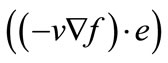
In this paper, we perform discussions on computational transport within a frame of linear theory. We propose a third-order computational method for numerical fluxes associated with the transport of a quantity f with a form of  in a direction e, where
  and ν are the velocity and diffusivity, respectively. The present scheme guarantees the positive difference coefficients of resulting finite difference equations for advection-diffusion equations in no use of any numerical flux limiter. Once we construct a stable scheme in a frame of linear theory, we apply it to nonlinear equations as well as linear equations in numerical experiments. Its evidence consists in the followings: We make use of an iterative calculation to take into consideration the nonlinear effect involved in nonlinear equations. In each iterative calculation at a given time step, a linear theory is applicable. This approach would be justified as long as its iterative solution converges. This is our policy. We confirm the convergence of iterative solutions in numerical experiments for nonlinear Burgers equation and discuss this justification.
Further we extend the present method into multi-dimensional equations. We perform numerical experiments for linear and nonlinear advection-diffusion equations to confirm the performance of the present scheme.
2. Mathematical Formulation
2.1. Numerical Stability
Regarding the numerical stability, we have the positive coefficient condition in a frame of linear numerical schemes that all coefficients linearly associated with the quantity f in the finite difference equations should be nonnegative. This positivty condition guarantees the stability such as monotone property of numerical schemes, monotonicity preserving condition, maximum principle, TVD (Total Variation Diminishing) condition and boundedness condition under the consistency condition of numerical schemes. Thus the positive coefficients condition with the consistency condition is sufficient condition for both the monotonicity and the boundedness of the numerical solutions.
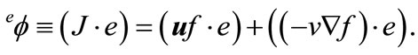
2.2. Transport Vector J and Numerical Flux 
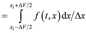
The transport vector J associated with a quantity f in a flow field  with the diffusion coefficient ν is expressed as
 (1)
(1)
where the first term and the second term denote the advection and the diffusion, respectively and νis the diffusion coefficient. The conservation low for f in case of no sources is expressed as
 (2)
(2)
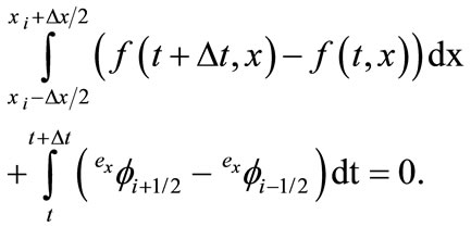
which corresponds to the advection-diffusion equation. By integrating Equation (2) over the time and space control volumes 
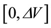 related to the computational cell under consideration and making use of Gaussian divergence theorem, we obtain
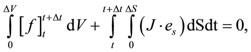 (3)
(3)
where es means the normal vector on the control volume surface. We define the numerical flux  in the direction e by
 (4a)
(4a)
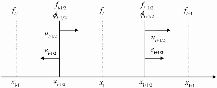
In case of one dimension shown in Figure 1(a), we have
 (4b)
(4b)
 (4c)
(4c)
where ex means a unit vector in the x-direction. Taking note of 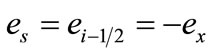 at
at  and
and 
 at
at , from Equations (3) and (4) we obtain in one dimension
 (5)
(5)
Hereafter we omit the superscript ex. In the first term in Equation (5) we approximate the averaged value of f over the control line  to be the value of f at the center of control volume, namely
 at any time t.
Further approximating the time integration in Equation (5) by the fully explicit scheme, we obtain the finite difference equation for the advection-diffusion equation by using numerical fluxes as follows:
 . (6)
. (6)
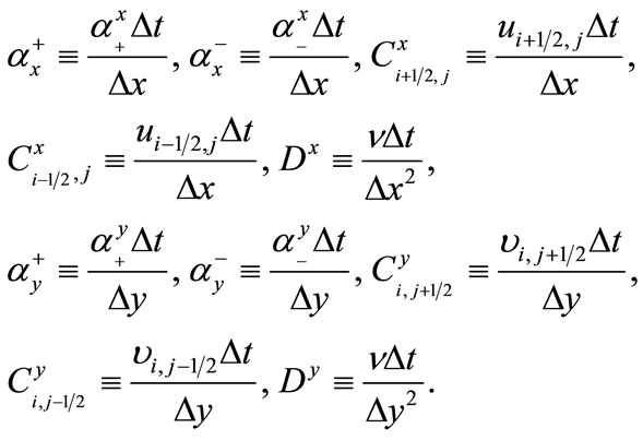
where the superscript n denotes the time step number and we let 
2.3. One-Dimensional Case
2.3.1. Finite Difference Equation
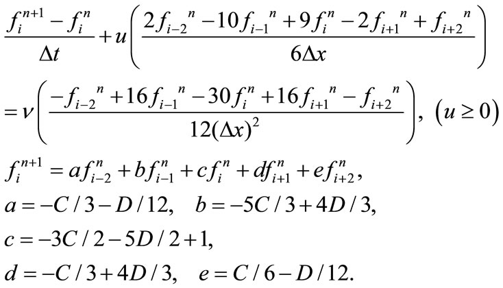
We perform a finite difference formulation for numerical flux . In the staggered grid with the velocity defined on the cell surface as shown in Figure 1, the quantity f and its derivative are to be interpolated using f at its surrounding cells. Here we perform mathematical formulation
 (a)
(a)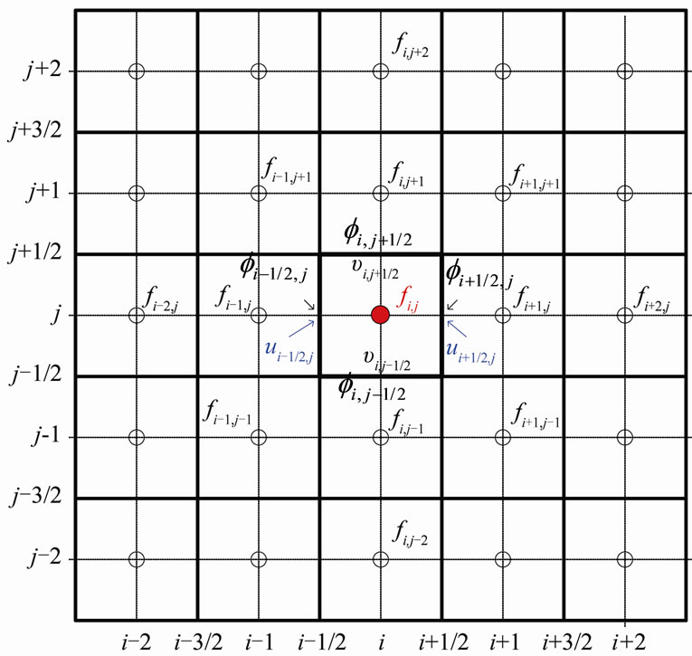 (b)
(b)
Figure 1. A computational grid. (a) One-dimensional grid, (b) Two-dimensional grid.
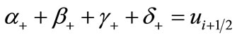
in case using 4 stencils to evaluate the numerical flux in one dimension. We expand  with respect to the cell surface point (i + 1/2) into the Taylor series. Taking a linear combination of those Taylor expansion series with multiplication of four parameters
  yields
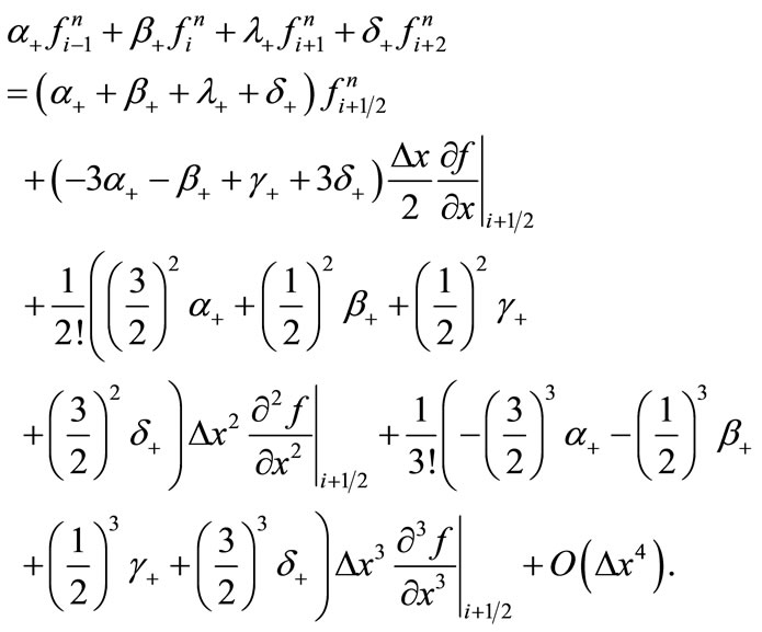 (7)
(7)
Requiring that the right-hand side of Equation (7) should be consistent with the numerical flux  given by Equation (4b) within the third-order accuracy, we obtain
 , (8a)
 (8b)
(8b)
 (8c)
(8c)
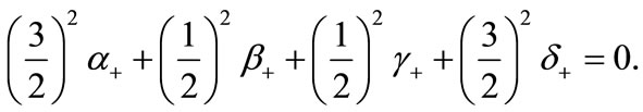
If we impose that the fourth term in the right hand side of Equation (7) is equal to 0, all parameters (
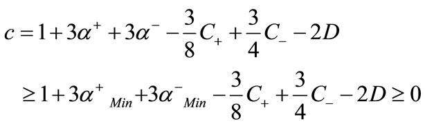
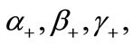 ) are to be determined uniquely. But in order to determine the difference coeffcients of the resulting difference equation so as to satisfy the stability condition (nonnegative condition), we solve the above three Equations (8a),(8b) and (8c) with a free parameter
  as follows:
 (9a)
(9a)
 (9b)
(9b)
 (9c)
(9c)
Thus we get
 (10)
(10)
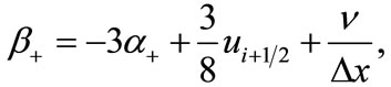
where  is the lowest-order term in the truncation errors defined by
 (11)
(11)
In the same manner as that in case of , we get
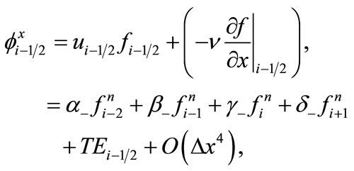 (12)
(12)
where
 (13a)
(13a)
 (13b)
(13b)
 (13c)
(13c)
 (14)
(14)
In the above equations two free parameters α+ and α- are to be determined later from the stability condition and requirement of minimum truncation errors.
Substituting Equations (10) and (12) into Equation (6) yields the finite difference equation:
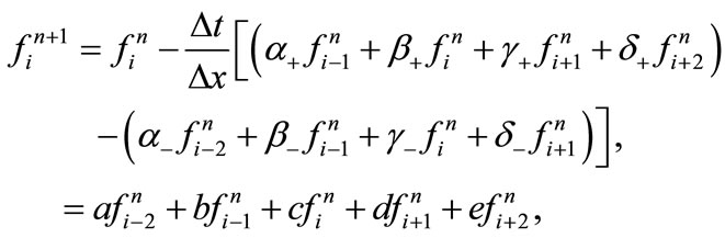 (15)
(15)
where
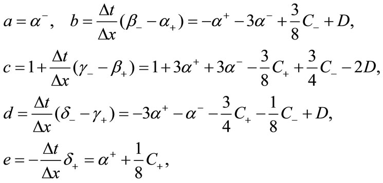 (16)
(16)
with 

2.3.2. Stability Condition
From the positive coefficients condition (rigorously nonnegative condition), we have the following stability condition:
 . (17)
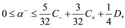
A solution of Inequalities (17) is given by (see Appendix A).
 (18)
(18)
 (19)
(19)
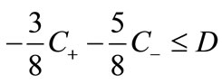
with the following additional conditions (see Appendix A):
 . (20a)
 , (20b)
 (20c)
(20c)
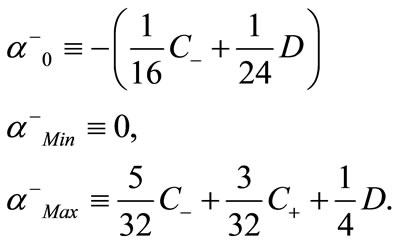
Inequalities(20a)-(20c) give an allowance domain for the Courant numbers (C+, C- ) and the diffusion number D, which is shown in Figure 2, where the allowance domain disappears as D goes to 0 corresponding to Godunov theorem.
Next, we determine the optimum values of ( ) at the local point
  so that the absolute value of truncation errors associated with the numerical fluxes may be minimum while keeping the allowance domain given by Inequalities(18), (19) and (20).
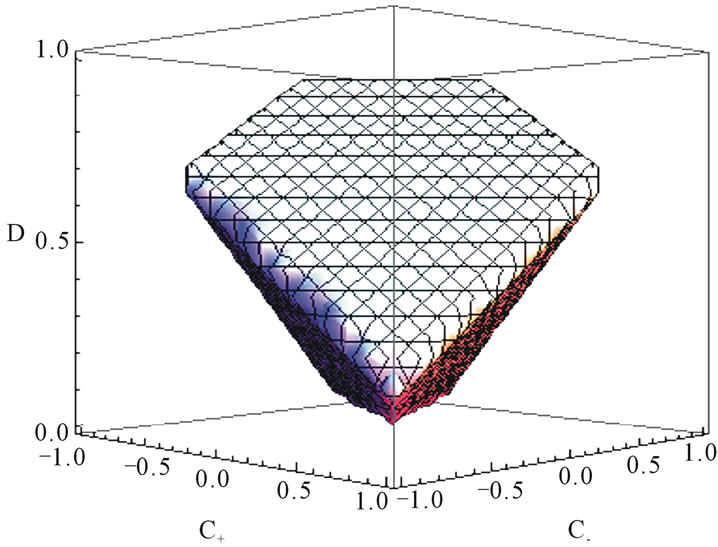
Figure 2. Stability domain in one-dimension.
2.3.3. Optimization
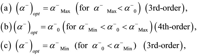
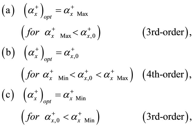
1) Optimum value of 
Here we consider the coefficient associated with  given by Equation (11). The absolute value of this coefficient is given by
 (21)
(21)
Under the condition given by Inequality(19), the optimum value  of α so as to minimize
  is classified by the following three cases:
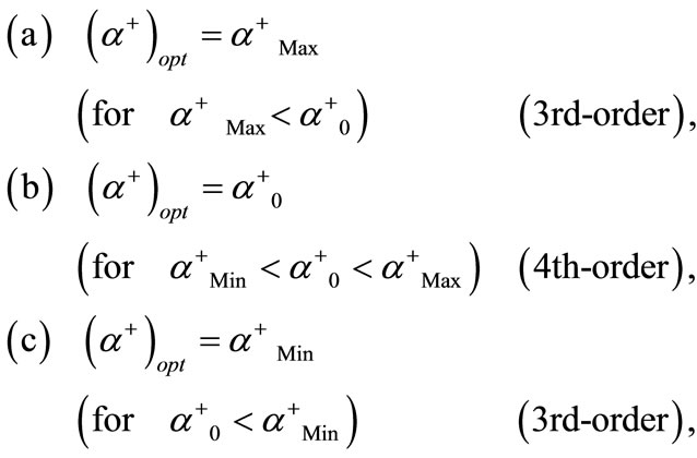 (22)
(22)
where
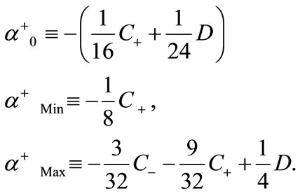
In case of (b),  becomes zero and the accuracy of
  turns up to the 4th-order.
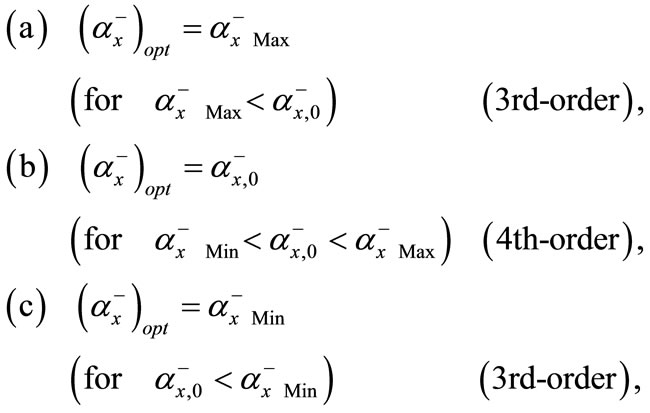
2) Optimum value of 
In the same manner as the case of , the optimum value
  of α so as to minimize the coefficient associated with
  is classified by the following three cases:
 (23)
(23)
where
2.3.4. Determination of 
From the stability domain given by Equations (20a) and (20b), the allowable space mesh increment  is determined by
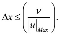 (24)
(24)
After the allowable space increment  is determined by Inequality (24), the allowable temporal increment
  is determined by using Inequality (20c) as follows:
 (25)
(25)
The allowable  and
and  given by Inequalities (24) and (25) depend on the diffusivity ν. If the diffusivity ν is small, which means convection-dominated flows,
  and
and  must be small according to ν. Thus the allowable
  and
and  determined by the above inequalities from the view point of numerical stability are to be small value in case of DNS (Direct Numerical Simulation), in which the diffusivity ν is the molecular viscosity and the small mesh increments
  and
and  are required to dissolve the small scale eddies from the physical point of view also. But in case of using a turbulence model based on a viscosity model with ν including the turbulence effect, considerably large values of mesh increments
  and
and  are to be allowed.
2.3.5. Accuracy for Temporal Term
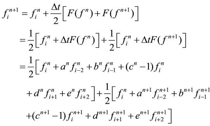
When we perform numerical calculations of advectiondiffusion equations, at least second-order schemes for the temporal term should be used. As long as the positive coefficients condition is satisfied at each Euler step in the second-order Runge-Kutta method or Crank-Nicholson scheme, the positivity condition can be maintained over the whole steps (see Appendex B). According to this fact, we employ the second-order Runge-Kutta method for linear equations and the Crank-Nicholson scheme for nonlinear equations, respectively in numerical experiments. We call this FLUX scheme.
2.3.6. Comparison with Conventional Schemes
We compare the present scheme given by Equations (15), (16), (18) and (19) with KAWAMURA scheme in a family of the conventional polynomial schemes in case of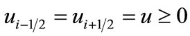 . Both schemes employ the same number 5 of stencils. Apply the KAWAMURA scheme and the fourth-order central scheme for the convection term and for the diffusion term, respectively, yields
The first coefficient  is always negative although the other coefficients can be positive. Thus the KAWAMURA scheme does not guarantee the positivity conditions, while the present scheme does the positivity of all difference coefficients.
2.4. Two-Dimensional Case
2.4.1. Finite Difference Equation
According to Equation (4a), the numerical flux in the direction ey is given by
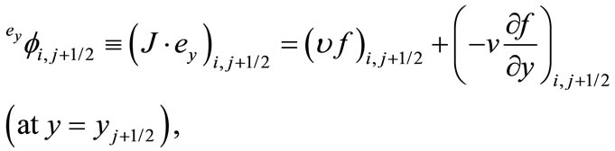 (26)
(26)
 (27)
(27)
where ey means a unit vector in the y-direction. Hereafter we omit the superscript ey. By making use of those fluxes and employing the same approximation for the time and space integrations as those used in one dimension, we obtain the finite difference equation for the two-dimensional conservation equation as follows:
 (28)
(28)
in which the averaged value of  over the control volume surface is approximated by the value of
  at the surface center such as:
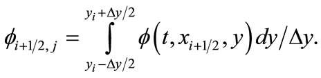
In the same manner as that in one dimension, we approximate  and
and  by using
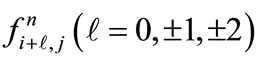
and , respectively. Then we obtain the finite difference approximation as follows:
 (29)
(29)
Here we have
 (30)
(30)
with the definition
In Equation (30),  is an arbitrary parameter. Here
  and
and  are adjusting parameters so as to minimize the truncation errors for
  and
and , respectively while keeping the stability condition. Further
  and
and  also are adjusting parameters so as to minimize the truncation errors for
  and
and , respectively while keeping the stability condition.
2.4.2. Stability Domain
From the positive (nonnegative) coefficients condition, we obtain inequalities such as
 (31a)
(31a)
 (31b)
(31b)
In a special case of ξ = 0, which would be enough in practical calculations, we can solve separately Inequalities (31a) and (31b). Consequently, in the same manner as that in case of one-dimensional equations, the solution of Inequality (31a) is given by
 (32a)
(32a)
 (32b)
(32b)
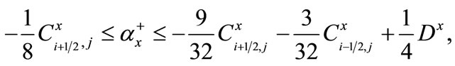
with the following additional conditions (the allowance domain for Cx and Dx):
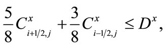 (33a)
(33a)
 (33b)
(33b)
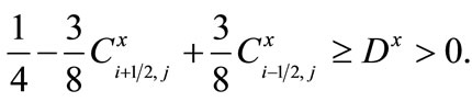 (33c)
(33c)
The solution of Inequality (31b) is given by
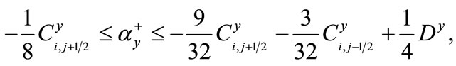 (34a)
(34a)
 (34b)
(34b)
with the following additional conditions (the allowance domain for Cy, and Dy):
 (35a)
(35a)
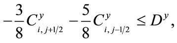 (35b)
(35b)
 (35c)
(35c)
The allowance domain for Cx and Dx given by Equation (33) is shown in Figure 3, in which CPX, CMX and DX denote ,
,  and
and , respectively.
2.4.3. Optimization
1) Optimum value of 
We consider the coefficient associated with the lowest
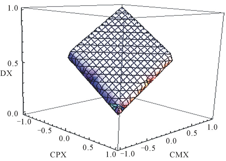
Figure 3. Allowance domain in two dimensions.
order term of truncation errors for the numerical flux . The absolute value of this coefficient is given by
 (36)
(36)
In the same manner as that in case of one dimension, the optimum value 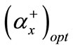 of
of  so as to minimize the coefficient
  under the condition given by Inequality (32a) is classified by the following three cases:
 (37)
(37)
where
 In case of 37(b), the coefficient of truncation errors becomes zero and the accuracy for the numerical flux
  turns up to the 4th-order.
2) Optimum value of 
In the same manner as the case of , the optimum value
  of
of  so as to minimize the absolute value of the coefficient associated with the numerical flux
  is classified by the following three cases:
 (38)
(38)
where
 In case of 38(b), the truncation error becomes zero and the accuracy for the numerical flux
  turns up to the 4th-order.
3) Optimum value of 
The optimum value of  so as to minimize the absolute value of the coefficients associated with the lowest order term of truncation errors is obtained by replacing the subscript or superscript x in Equation (37) with y.
4) Optimum value of 
The optimum value of  so as to minimize the absolute value of the coefficients associated with the lowest order term of truncation errors is obtained by replacing the subscript or superscript x in Equation (38) with y.
In the same manner as that in case of two-dimensional equations, we can straight-forwardly extend our optimized scheme into three-dimensional equations.
3. Numerical Experiments
3.1. One-Dimension
3.1.1. Linear Advection-Diffusion Equation
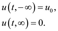
When the initial distribution is given by  in an infinite region and the boundary values at
  are zero, the analytical solution of Equation (2) with the constant velocity u is given by the following Gaussian distribution:
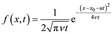 (39)
(39)
We employed the total cell number N = 100. The Courant number and diffusion number are C = 0.1 and D = 0.1, respectively. We set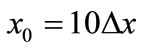 . As the initial condition for numerical experiments, we use the Gaussian distribution given by Equation (39) with
 , in which
  is multiplied to Equation (39) to make the solution be non-dimensional. The boundary conditions are
 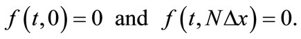 Hence we limit the computational time so that this boundary condition is consistent with the exact solution. We employ the secondorder Runge-Kutta method for the time discretization. Figure 4 shows the numerical solutions with the analytical solution at the time step number n = 100, 300 and 600. The present scheme shows good solutions free from numerical oscillations.
3.1.2. Nonlinear Burgers’ Equation
In one dimension, Burgers’ equation is
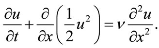 (40)
(40)
We separate the flux term  in Equation (40) into
  and count
  as a transport velocity on the computational cell surface, which is approximated as an averaged value between the adjacent cells, namely
  on the surface between the cell i and the cell
 . We employ
 and
and 
 , where
  is a reference velocity. For the time discretization, we employ the second-order CrankNicholson scheme.
1) Shock wave propagation problem
We solve Equation (40) under the initial condition at t = 0:
 (41)
(41)
and the boundary conditions at :
:

Figure 4. Comparison of numerical solutions with the analytical solution.
 (42)
(42)
At t = 0 the shock wave is located at x = 0. For this combination of initial and boundary conditions, Equation (40) has the exact solution given by
 , (43)
where exp and erf denote the exponential function and the Gaussian error function, respectively.
In numerical experiments, the boundary condition u(t, x) = 0 at x = 100Δx is employed. Hence we limit the computational time so that this boundary condition is consistent with the exact solution.
a) Convergence check
For the time discretization, we employ the secondorder Crank-Nicholson scheme, whose computational algorithm is simple and convenient for iterative calculations to take account the nonlinear effect involved in Burgers’ equation. Namely, the difference coefficients (a, b, c, d and e) given by Equation (16) depend on u and are updated in each iterative calculation at every time step until the solution converges. In this connection with the discussion in Introduction, our policy for the application of a scheme based on a frame of linear theory to nonlinear equations is justified as long as the numerical solution converges in iterative calculations at every time step. Hence we check this convergence .
We continue the iterative calculations at each time step number n until the relative error of solutions reaches the pre-asighned limit ε for all spatial mesh numbers i; namely:
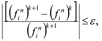 (44)
(44)
where k denotes the iteration step number. In actual calculation, a small value 10–20 is added to avoid the denominator being zero. Figure 5 shows the iteration numbers for ε = 10–6, 10–8, 10–10 and 10–12 at the time step number n = 1-100. The calculation were performed on Fortran Compiler by using double precisions. In the following numerical experiments, all numerical solutions converged.
b) Results
Figure 6 shows the comparison of numerical solutions with the exact solution at time step number n = 500, 1000, 1500. The numerical solutions with the present FLUX scheme are free from numerical oscillations and are in good agreement with the analytical solution.
2) Steep gradient formation problem
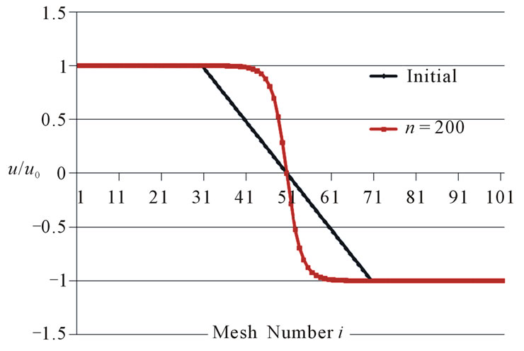
In Figure 7, initially the velocity u is zero at the origin x = 0 and the quantity u propagates toward the origin x = 0 from both right and left outsides, resulting in forming a steep distribution of u at the origin. Figure 7(b) shows the result after a lot of elapsed time n = 10000, in which the advection of quantity u is almost balanced to its diffusion and the solution attains to an almost steady state.
When the diffusivity ν goes to 0, Burger’s equation approaches an advection equation, which may include many weak solutions inclusive of an upright wave for this initial condition. The present FLUX scheme needs nonzero diffusivity and is not applicable to such pure advection equation. But a vanishing viscosity approach using the present scheme would be available and we could expect to get a unique and physically relevant solution among many weak solutions.
3) Rarefaction wave propagation problem
In Figure 8, initially the velocity u is zero at the origin x = 0 and the quantity u propagates toward the both outsides (x = 0 and x = 100Δx) from the inside, resulting in forming a rarefaction wave. Figure 8 shows the result at
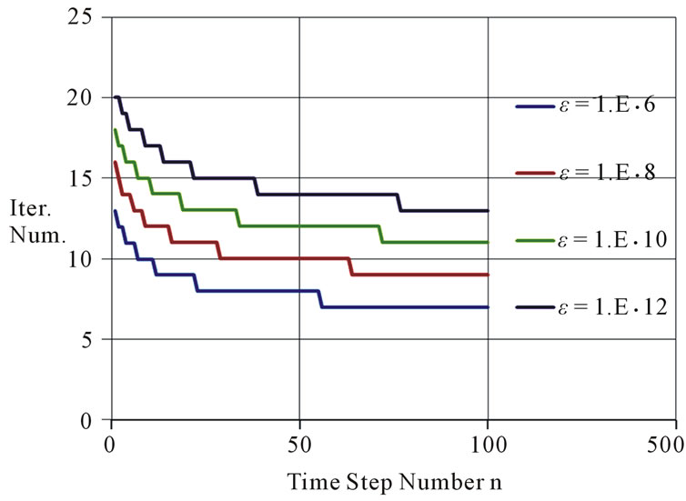
Figure 5. Convergence check in iterative calculations.
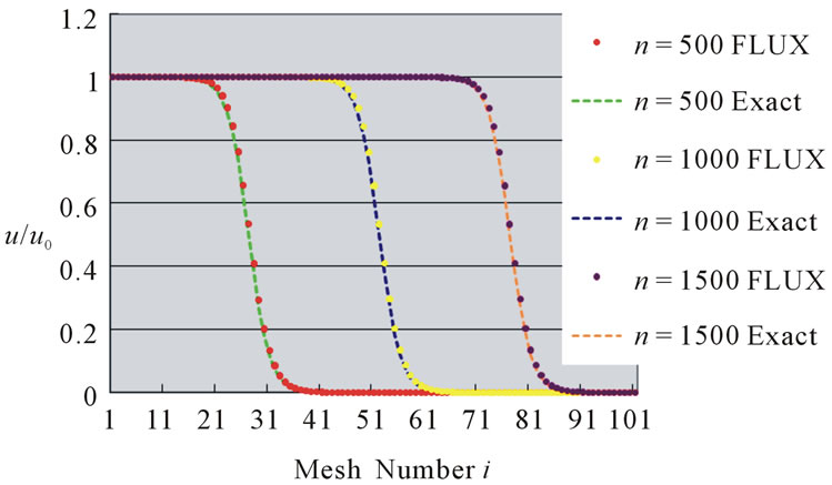
Figure 6. Comparison of solutions with analytical solution for nonlinear Burgers’ equation.
 (a)
(a)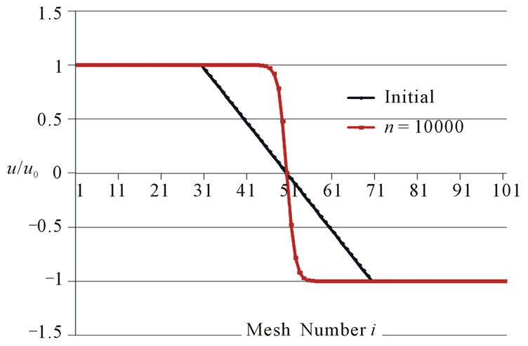 (b)
(b)
Figure 7. Solution for steep gradient formation.
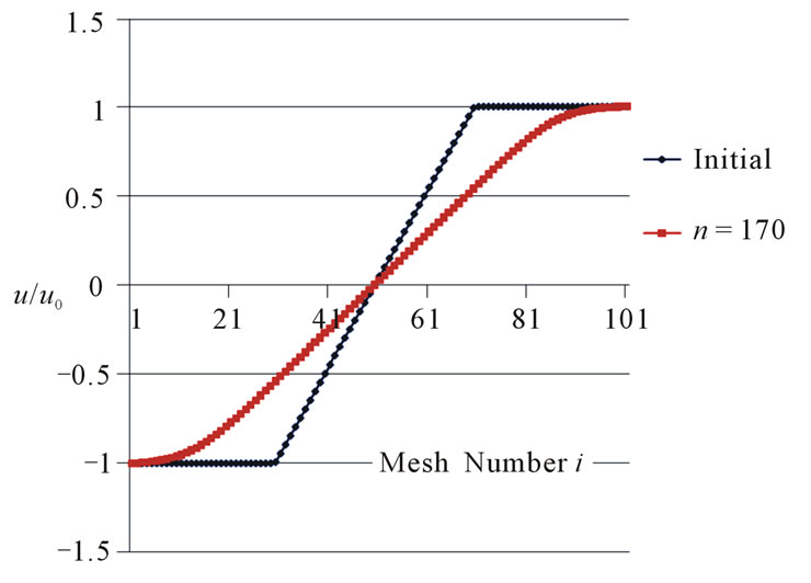
Figure 8. Solution for expansion wave.
n = 170. All numerical solutions obtained in the above numerical experiments are free from numerical oscillations.
3.2. Two Dimensions
We solve a two-dimensional advection-diffusion equation given by Equation (2). Figure 9 shows the computational geometry and the boundary conditions. We employed a computational cells 50 × 50 with uniform meshes and Dirichlet boundary conditions on all boundaries. Namely, f = 0 on the bottom and right boundaries and f = 100 on the left and top boundaries. Outside the boundaries, the same values as those on each boundary are set at mesh points near the boundaries. Hence any special treatment near the boundaries is not necessary, resulting in keeping the third-order accuracy all over the computational domain. We would rather focus to confirm the monotonicity properties of solutions with the present 2-D scheme. Initially, the values of f are set 0 all over the inner domain. Thus, the solution of this problem approaches a stationary solution. The velocity distribution is uniform, and the Courant numbers and the diffusion numbers are Cx = Cy = 0.1 and Dx = Dy = 0.1, respectively. These values satisfy the 2-D allowance domain of C and D given by Inequalities (33a), (33b) and (33c).
Both solutions with the KAWAMURA scheme and the UTOPIA scheme suffered from the numerical instability and diverged at a few time steps. The present 2-D optimized scheme showed stable solutions in Figure 10(a) at the time step number n = 500, and in Figure 10(b) along a diagonal line with  at n = 100, 200, 300 and 500. The solution along a diagonal line at n = 300 is almost same as that at n = 500, which seems to approach the stationary solution.
4. Conclusions
We discussed higher-order computational schemes for numerical flux  with a form of
 in a direction e within a frame of linear theory. We proposed a third-order polynomial scheme for numerical fluxes to guarantee the positive difference coefficients of resulting finite difference equations for
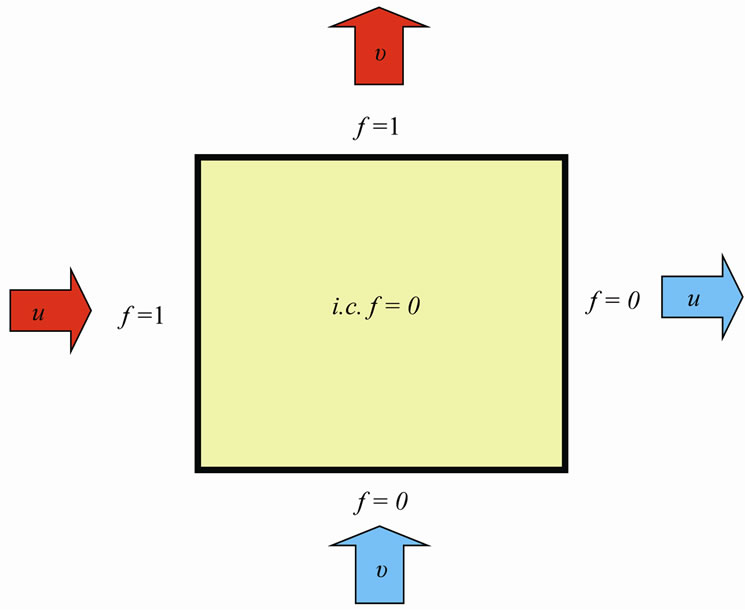
Figure 9. Computational domain and boundary conditions.
 (a)
(a)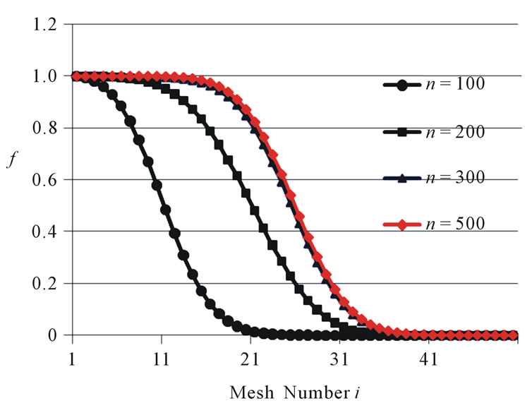 (b)
(b)
Figure 10. Solution for 2-D advection-diffusion equation. (a) Distribution in 3-D view at n = 500. (b) Distribution along the diagonal line.
advection-diffusion equations. We found a function to regulate the positivity of the numerical scheme in terms of local Courant numbers and diffusion numbers and to optimize the scheme with respect to the numerical stability and the truncation errors. The feature of the present optimized scheme consists in keeping the third-order accuracy anywhere without any numerical flux limiter by using the same stencil numbers as conventional thirdorder schemes such as KAWAMURA and UTOPIA schemes.
Further, we extended the present method into multidimensional advection-diffusion equations. We performed numerical experiments for linear and nonlinear Burger’s equations taking account the feedback of nonlinear effects in iterative calculations, resulting in numerical solutions free from unphysical oscillations.
5. References
- B. P. Leonard, “A Stable and Accurate Convective Modeling Procedure Based on Quadratic Upstream Interpolation,” Computer Methods in Applied Mechanics and Engineering, Vol. 19, No. 1 1979, pp. 59-98. doi:10.1016/0045-7825(79)90034-3
- T. Kawamura and K. Kuwahara, “Computation of High Reynolds Number Flow Around a Circular Cylinder with Surface Roughness,” Fluid Dynamics Research, Vol. 1, No. 6, 1986, pp. 145-162. doi:10.1016/0169-5983(86)90014-6
- M. Chapman, “FRAM Nonlinear Damping Algorithms for the Continuity Equation,” Journal of Computational Physics,Vol. 44, No. 1, 1981, pp. 84-103. doi:10.1016/0021-9991(81)90039-5
- A. Harten, “High Resolution Scheme for Hyperbolic Conservation Laws,” Journal of Computational Physics, Vol. 49, No. 3, 1983, pp. 357-393. doi:10.1016/0021-9991(83)90136-5
- K. Sakai, “A Nonoscillatory Numerical Scheme Based on a General Solution of 2-D Unsteady Advection-Diffusion Equations,” Journal of Computational and Applied Mathematics, Vol. 108, No. 1-2, 1999, pp. 145-156. doi:10.1016/S0377-0427(99)00107-7
- K. Sakai and I. Kimura, “A Numerical Scheme for Compressible Fluid Flows Based on Analog Numerical Analysis Method,” Computational Fluid Dynamics Journal, Vol. 13, No. 3, 2004, pp. 468-482.
- K. Sakai and I. Kimura, “A Numerical Scheme Based on a Solution of Nonlinear AdvectionDiffusion Equations,” Journal of Computational and Applied Mathematics, Vol. 173, No. 1, 2004, pp. 39-55. doi:10.1016/j.cam.2004.02.019
Appendix A
From the positive coefficients condition (nonnegative condition), we have the following stability condition:
 . (A-1)
We let the minimum value of  be
be , the maximum value of
  be
be , the minimum value of
  be
be  and the maximum value of
  be
be . Once we find
 ,
,  ,
,  and
and  in terms of
  ,
,  and D, we obtain the solution for Inequality (A-1) as follows:
 (A-2)
(A-2)
 (A-3)
(A-3)
From Inequalities (A-2) and (A-3) and Equation (16), we get
 (A-4)
(A-4)
 (A-5)
(A-5)
 (A-6)
(A-6)
 (A-7)
(A-7)
 (A-8)
(A-8)
From Inequality(A-4), we obtain
 (A-9)
(A-9)
From Inequality(A-8), we obtain
 (A-10)
Applying Inequalities(A-9) and (A-10) into the righthand side inequality in Inequality(A-6) yields
 (A-11)
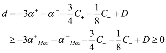
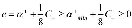
The right-hand side inequality in Inequality (A-11) is one of the allowance conditions among C+, Cand D.
If we replace the right-hand side inequality in the above Inequalities (A-5) and (A-7) with equality, we get simultaneous equations with respect to , and
, and  as follows:
 (A-12)
 (A-13)
From Equations (A-12)-(A-13), we obtain the solutions
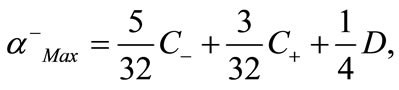 (A-14)
 (A-15)
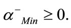
Although  and
and  given by Equations (A-14) and (A-15), respectively are one of the solutions for Inequalities (A-5) and (A-7), these solutions surely satisfy the second and fourth Inequalities (A-1), namely (
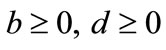 ). Namely, Equations (A-14) and (A-15) are the sufficient solution to guarantee
  and
and .
.
Combining Inequalities (A-2) and (A-3) and Inequalities(A-9) and (A-10) with Equations (A-14) and (A-15), we obtain the formal solutions for the stability conditions given by Inequality(A-1) as follows:
 (A-16)
 (A-17)
with an additional condition of the right-hand side Inequality in Inequality(A-11)
 (A-18)
In order for Inequalities(A-16) and (A-17) to hold substantially, the right-hand side equations of those Inequalities must be greater than each of the left-hand side equations. From this requirement, we obtain
 (A-19)
 (A-20)
Inequalities (A-18), (A-19) and (A-20) are the additional conditions among C+, Cand D.
In conclusion, Inequalities (A-16) and (A-17) with the additional allowance conditions given by Inequalities (A-18), (A-19) and (A-20) give a sufficient solution to guarantee Inequality(A-1).
Appendix B
An advection-diffusion equation in one-dimension is expressed by
 (B1)
(B1)
 (B2)
(B2)
Discretizing Equation (B1) by using the CrankNicholson scheme and Equation (B2) by using the present FLUX scheme yields
 (B3)
(B3)
In Equation (B3),  are the difference coefficients evaluated at the time step n + 1 and calculated iteratively based on the values at earlier iteration step at the same time step n + 1 untill
  is converged within a pre-asighned value εgiven by Equation (44). From Equation (B3), we obation
 (B4)
(B4)