ABSTRACT

We develop a multi-period dynamic model in which managers decide in each period how much to invest in improving process reliability. The optimal investment decision will minimize the firm’s total costs, which are comprised of its preventive costs and failure costs. We explicitly characterize the optimal investment scheme under different output growth projections and where the firm considers project obsolescence and investment salvageability. Our findings include: for sufficiently small output growth, investment will be made upfront; for sufficiently large output growth, investment will be made periodically until project termination; and for intermediate growth, investment will be staged until some period after which there will be no more investment. The general nature of the cost function in this model allows for its application in various cost reduction settings.

1. Introduction

Firms make many investments in attempt to prevent failure costs or, at least, to minimize those costs. These investment decisions are made frequently, and repeatedly as the costs they seek to prevent are ever recurring. For example, firms invest in improving production processreliability to avoid costs associated with faulty products. When a defective product gets to the marketplace then the producers incur not only operational costs such as the need to fix the production line and reproduce or repair the product but also marketing costs (reputation losses, advertisement), logistical costs (recall the product, distribute replacements and parts) and legal costs (lawsuits and settlements). Considering, for example, the automotive industry, which is beleaguered with tremendous costs associated with recalls [1], with approximately 30 million vehicles recalled, auto-makers in the US spent more than 3 billion dollars in 2004 alone on direct recall costs [2]. These considerable failure costs make it extremely important for firms to follow an investment policy that optimally balances between the sums of money that are invested and the savings received by those investments.

In this paper, we model a dynamic investment scheme in which investment decisions are made periodically to minimize costs. The firm experiences time-dependent periodical costs that may be reduced through investment. The project terminates at some finite time after which investments may be (partially) salvageable. At each period during the project’s planned life, a catastrophic event may occur in which the project and its technology become obsolete. In case of obsolescence, the future costs and the salvage value of past investments are zero.

We derive the unique optimal investment policy for each period in the planning horizon. In particular, we find that when the growth of costs is sufficiently high, depending on the probability for obsolescence and the inter-temporal discount rate, investment is installed over time. When the growth rate of costs is low, depending on the probability for obsolescence, the planning horizon, the inter-temporal discount rate and the salvage ability of investment, it is optimal to invest upfront. Finally, medium growth investment will be made sequentially until some intermediate period after which there will be no more investment.

The general nature of the cost function in this model allows for its application in various cost reduction settings. For example, the model may be applied for deriving optimal training schedules of employees. Investment in training the employees is economically justified due to the savings that are attained by better trained personnel. However, the optimal timing and the extent of this training must be derived in order to maximize total savings.

Our choice for a general cost function follows the established research field of quality related costs, recently reviewed by [3]. Foster [4] categorizes quality associated costs into three groups: Prevention costs, Appraisal costs, and Failure costs. Similarly, Feigenbaum [5] suggests two broad categories for costs, namely, quality improvement costs and losses due to poor quality. Indeed, research clearly indicates that the quality related cost function cannot be simply brushed off with some specific functional form. Accordingly, we make only nonrestrictive assumptions on the cost function to guarantee a unique optimal solution. This allows us to admit a wide variety of cost function forms suggested by theoretical research and practical examples.

The allocation of preventive costs is investigated by researchers in various contexts. Gilardoni and Colosimo [6] explore the optimal timing of preventive maintenance. Freimer et al. [7] describe how quantity production decision is affected by quality improvement when defects are possible. The focus of their work is the balance between production quantity and quality. Freiesleben [8] analyzes optimal allocation of quality inspection systems in a single period model. Fine and Puertos [9] firms dynamically invest in improving process quality and setup reduction. Their model includes uncertainty as to the degree of improvement that may be attained in each investment period. They find that investment is made until a target level of quality is attained. Examining the tradeoff between investment in quality with investment in productivity, [10] considers how the firm maintains its demand and competitive advantage. In contrast to [10], we do not consider the effects of quality on demand of the product. The focus of our paper is on the effects of growth on investment. Therefore we assume that growth is an exogenous decision by the firm and do not consider the role of quality in expanding the firm’s competitive edge.

Another strand of research in this field focuses upon the interaction of learning and quality costs. This research includes theoretical papers such as [11-13]. The latter balances between investment in knowledge creation and future payoffs from this knowledge, while considering capacity losses due to investment. Empirical papers in this field include [14,15]. Ittner et al. [15] find that past failures motivate firms to increase their future quality through what is called autonomous learning. We follow the line of [10,16] in assuming induced learning, (i.e. learning is induced by investments), and disregard the learning effects of past failures.

2. The Model

Consider a risk-neutral firm that owns a production project with a T-period operation horizon. The firm incurs costs associated with the reliability of its production process and therefore considers investing in improving its reliability in order to minimize costs.

2.1. Reliability

The key state variable in the model is the firm’s process reliability, , which is a proxy for the production process’s level of reliability or quality during the i’th period,. The more reliable the production process the less faulty products will be produced and consequently the firm incurs lower failure costs. The firm can invest in improving its process reliability. Specifically, let denote the initial reliability. If the firm invests dollars at the beginning of the i’th period then the reliability during the period is given by

(1)

2.2. Salvage Value of Investment

We assume that following the last period the project is consolidated and all investments in the project are salvaged at dollars per dollar invested1. Prior to termination, however, investment cannot be salvageable; that is, the firm cannot extract any capital from its already invested reliability and therefore investment in each period is nonnegative. Investment can only be salvaged following termination because past investments cannot be disentangled from the production process and their extraction negatively impacts the project. Conversely, once the project is terminated the firm can salvage its past investments without incurring any project-related costs. In the event of obsolescence, investments have zero salvage value. Without loss of generality we assume that the initial reliability, , is salvageable, too.

2.3. Periodical Costs

At any period, i, the firm expects that a portion of its output will be defective and that as result it will incur related costs such as operational, marketing, logistic and legal costs. Let c_i denote the costs at period i. We assume that c_i is the product of three factors as explained below:

(2)

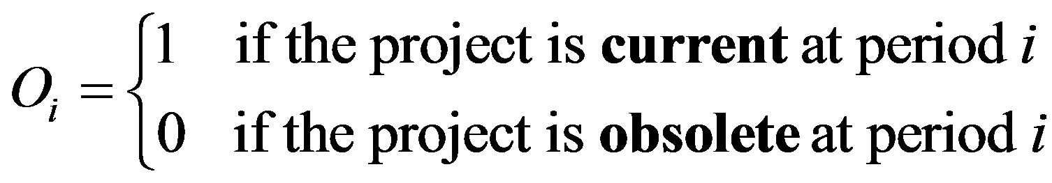
• Obsolescence: The project is subject to the risk of obsolescence. For example, in the event of the development of a technology superior to the project’s technology the firm’s top management may decide to terminate all operations associated with this project. is an indicator function determining the obsolescence status of the project, where

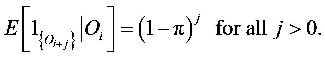
Obviously, once a project is obsolete it stays in this status forever. Let, denote the probability for a current project to turn obsolete in the next period. We also assume that the probabilities to turn obsolete are independent between periods. Hence, a project stays current in the next period with probability and we have that

Since all operations are terminated once the project is obsolete, in particular, the firm bears zero costs from an obsolete project, hence the formulation given in (2). Finally, we assume that the catastrophic event leading to obsolescence happens at the end of each period after all the current period’s costs were realized.

• The Effect of Reliability: Improving the production’s line reliability serves to reduce the portion of faulty output and therefore the firm’s costs decrease with reliability. Thus, is assumed to be a decreasing function. To guarantee the existence of a unique solution we additionally assume is continuously differentiable, convex, and .

• Cost Factor: It is assumed that failure costs are positively correlated with the production size. More specifically, we assume that if reliability does not improve, costs grow at a fixed rate between periods. This growth models three possible economical phenomena: 1) Growth in the firm’s production (i.e. periodical output) and as an immediate consequence, growth in the periodical costs; 2) Depreciation in the process reliability and therefore, without improving reliability costs will grow; 3) Increase in consumer sensitivity to quality and safety and growth in governmental oversight2. The cost factor at period i, , is given by

, (3)

where α > 0 is the growth parameter and is the initial cost factor.

2.4. Timing of Events

The firm’s intertemporal discount factor is denoted by. For discounting purposes, we assume that investments and costs are incurred at the beginning of each period and that the savings from salvaging investment are received at the beginning of the period following the last.

3. The Optimal Investment Policy

The optimal investment policy at each period depends on whether a catastrophic event leading to obsolescence has occurred. We therefore begin our analysis by examining the firm’s optimal decision in the last period, contingent on the project still being current (i.e. non-obsolete) and then go inductively backwards in time until the first period.

3.1. Period T

Immediately before the last period, the firm’s reliability is given by. Given that the project has survived thus far, i.e. the technology is not obsolete, the firm must decide its investment so to minimize its total expected costs and therefore the T period problem is

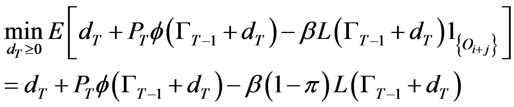(4)

In (4), we consider costs and therefore the last expression, which represents the savings from salvage, is negative.

From cost perspective, obsolescence can be subsumed by adjusting the discount factor. Therefore, for the purpose of mathematical presentation we may define as the obsolescence-adjusted discount rate and set

.

The following lemma is useful for the characterization of the optimal solution.

Lemma 1:

Let. The unique solution to, denoted, is positive and increasing with.

Proof: To simplify exposure we provide proofs in the Appendix.

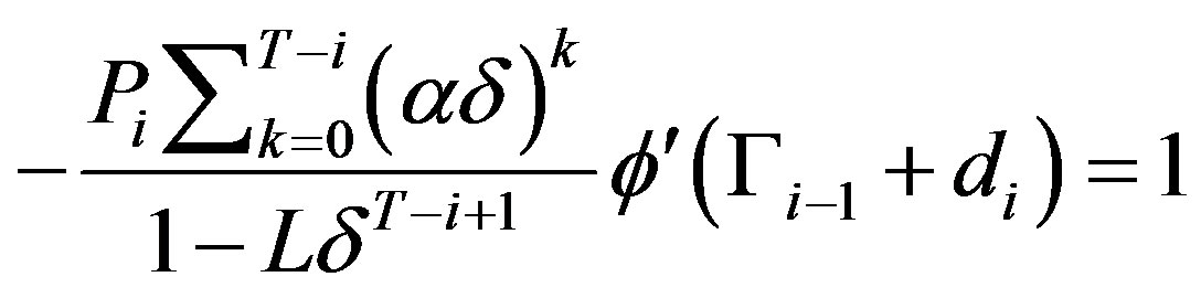
First order condition of the firm’s problem, (4), is given by

.

Since, however, , by Lemma 1 the optimal investment in the last period is

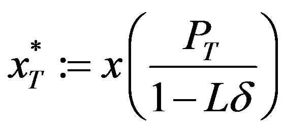
where we use the notation.

Let

thus

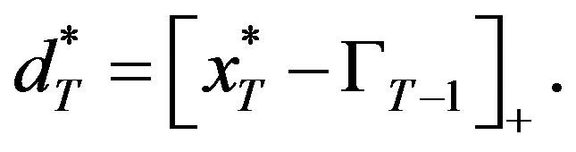(5)

We find that in the last period, if the project is current the optimal investment policy is a threshold policy. If is below the threshold level, , investment will be made so that the quality will reach the threshold level. Otherwise, there will be no investment.

3.2. Period T − 1

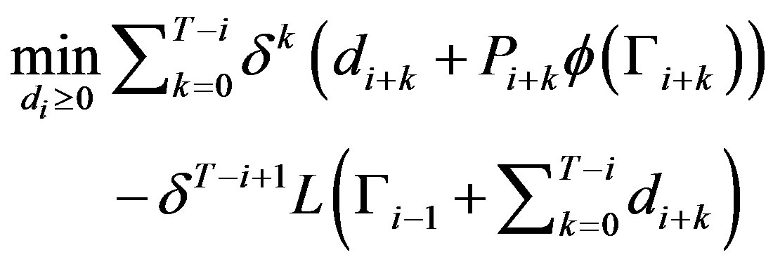
The analysis continues inductively backwards in time until the first period. To motivate the inductive argument we demonstrate the solution for period, after which the inductive argument will be made. At period, if the project is not obsolete, the firm’s problem is to minimize its total expected amortized costs

Substituting (1), (3) and (5), we have the firm’s problem:

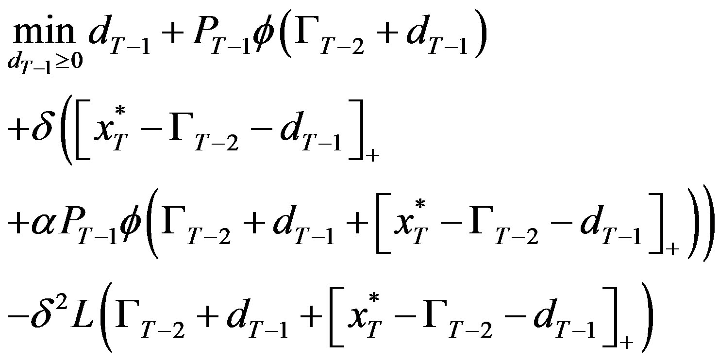(6)

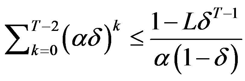
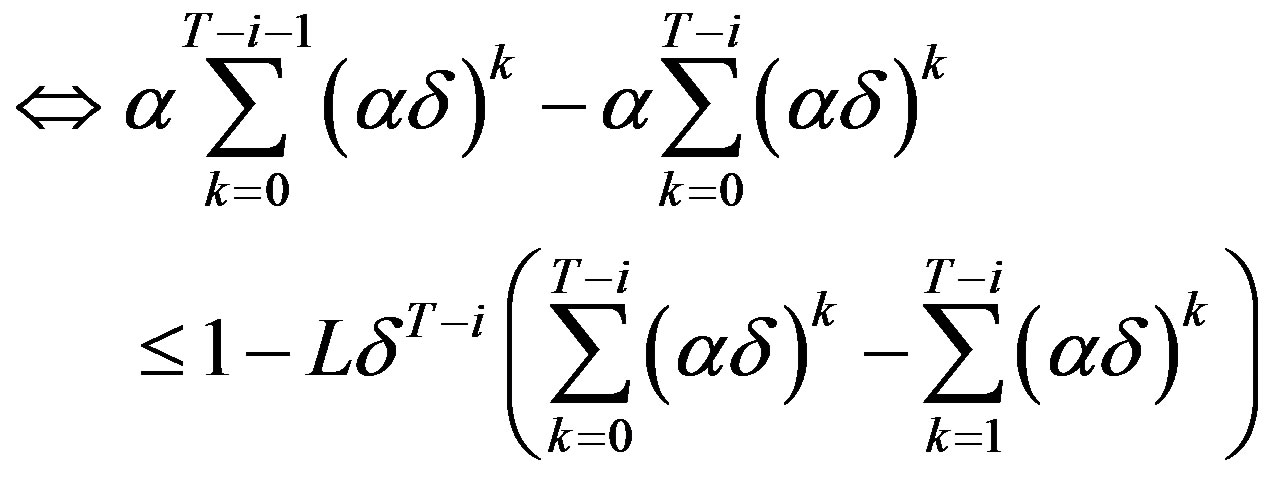
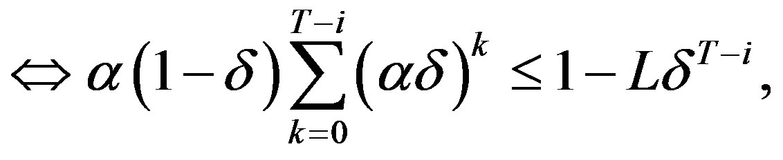
Case 1::

Now,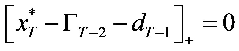 for all and therefore the firm’s problem, (6) can be written as

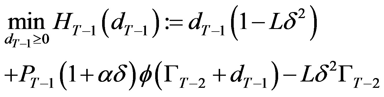
Case 2::

The firm’s problem, (6), is given by

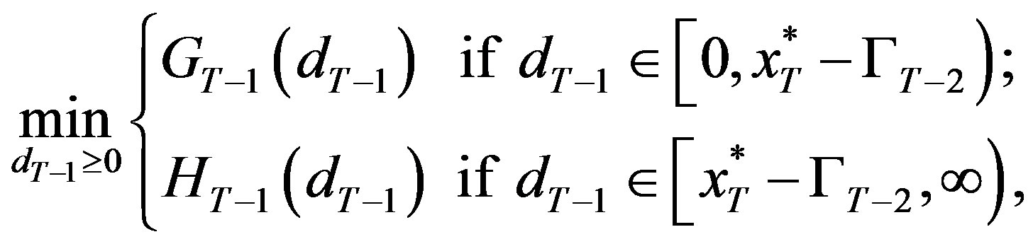
where

Proposition 1:

If the project is current at period T − 1 then the optimal investment policy at the period is a threshold policy,

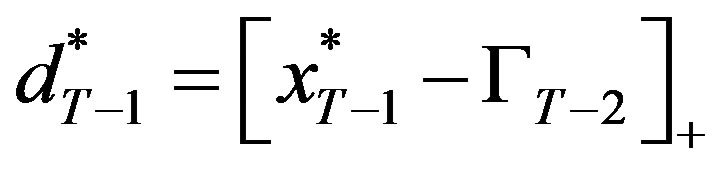
where the threshold level, , depends on the output’s rate of growth, α, in the following manner:

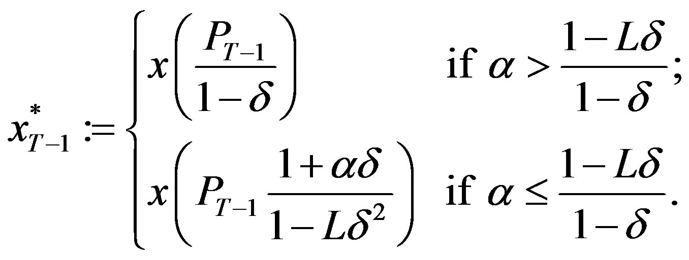
Notice that when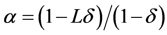, then

and so the threshold level is continuously non decreasing in α with an upper bound

We interpret the investment policy in period as follows: In general, future costs affect the current investment decision and therefore higher future costs (i.e. higher) will result with increased current investment to mitigate those costs. However, for sufficiently high future costs saturation is achieved and any additional increase in future costs will not affect the current optimal investment decision.

3.3. The Inductive Argument

Proposition 1 states that the threshold policy for period may be one of two forms, depending on the value of. The inductive argument will assume that at each future period we have indeed a threshold policy and that the threshold value may take one of two forms. Formally, is defined as the first date, , to meet the condition

(7)

if such a date exists, i.e. if condition (7) is met before the last period. Otherwise,.

Lemma 2:

For any period, condition (7) is met strictly.

Lemma 2 guarantees that all periods beginning with satisfy (7) and that all periods prior to do not satisfy it. We now turn to state the central result of the paper:

Theorem 1 (Optimal Investment Policy):

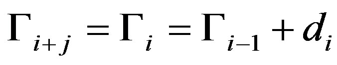
The optimal investment policy in each period, is given by, where

As long as the project is current, investment will take place according to a threshold policy where is the threshold level. In the following section we discuss the implications of Theorem 1 on the investment path.

4. Discussion

At each period, the firm’s investment is bounded by the threshold level. We begin our discussion in characterizing the threshold level.

Proposition 2:

The threshold level at each period, i is non-decreasing in and bounded above by

If is such that it can be easily see from the definition of and Lemma 1 that the threshold level is increasing in. Proposition 2 determines that, nevertheless, investment is bounded. That is, investment increases with until a critical growth level after which investment is fixed at A further increase of will not affect the threshold level.

The actual investment in any given period, however, depends not only on the current period’s threshold level but also on earlier threshold levels. For example, if the previous period’s threshold level is higher than the current period level, then in the current period the optimal investment level is zero. In contrast, when the previous periods’ thresholds are lower than the current threshold, investment will be such that it will increase reliability to the current threshold. Thus, to derive the optimal investment policy we need a characterization of the threshold trajectories over time. This is the subject of the following proposition.

Proposition 3 (Output Growth):

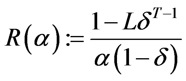
Let and let denote the unique solution to

(8)

a).

b) Low Growth: If then and the threshold levels are non-increasing between the first and second period and decreasing thereafter.

c) Medium Growth: If then and the threshold levels are increasing until, nonincreasing between and and decreasing thereafter.

d) High Growth: If then and the threshold levels are increasing.

Proposition 3 groups the possible growth rates intothree distinct, non-empty groups, each characterized by a different threshold trajectory. This result balances between the advantages of postponing investment and the value added by capturing as many periods of savings as possible. Consider, for example, when there is zero growth. Since costs are identical in each period (for the same level of reliability), then the earlier periods “see” more periods of identical savings and therefore will justify higher investment. Thus, the threshold level will decrease over time as there are less savings to gain. In contrast, when growth is positive, later periods see significantly higher costs than early periods. If growth is sufficiently high, these extra costs more than offset the effect of the shorter horizon seen by later periods. Therefore, for sufficiently high growth the threshold levels are increasing. Moreover, the critical point at which we will prefer to invest gradually is the point where the current investment captures an infinite horizon, i.e.. Since we can not capture savings from any more periods, if required, investment is made in the next period.

The varying nature of the threshold trajectories described in Proposition 3 dictates different optimal investment trajectories, as described in the next theorem.

Theorem 2 (Optimal Investment Path):

a) When growth is low: If the firm will not invest in improving its reliability. Otherwise, the firm will invest in the first period and will make no additional investments.

b) When growth is medium: If the firm will not invest in improving its reliability. Otherwise, if the project is still current, the firm will begin investing in the first period whose threshold is greater than. Investment will be made in every period, contingent on the project being current, until period, after which there will be no further investment.

c) When growth is high: Contingent on the project being current, the firm will begin investing in the first period whose threshold is greater than and will continue investing in each period after that.

5. Sensitivity to the Planning Horizon (T)

Next, we examine the effect of the size of the planning horizon on the optimal investment policy.

Proposition 4:

a) The critical date, , is non-decreasing in T.

b) is decreasing in T.

c) The threshold levels at the critical date and later are increasing in T.

Investment increases with the planning horizon because the savings to be made from the additional periods justify additional investment. While this result is intuitive, the exact manner in which it increases, however, is less intuitive. The implication of Proposition 4 is that the increased investment happens through either or both of the following two ways: 1) Increasing the investment level at the critical date; 2) Delaying the critical date, thus allowing additional investment periods. By Proposition 2 the investment in the critical date will grow at most to. If additional investment is needed, it will happen by increasing the critical date and adding an additional investment period.

6. Sensitivity to the Salvage Factor (L)

Proposition 5:

a) The critical data, , is non decreasing in L.

b) and are decreasing in L.

c) The threshold levels in period are increasing in L.

The threshold levels are increasing in L since as the firm can salvage a higher percent of its investment, the “cost” of investment is lower relative to the savings that are achieved. The consequence of Proposition 5 is that increasing salvage ability has a similar effect on investment than increasing the planning horizon. By increasing salvage ability investment increases through (1) more investment in the critical date and (2) the increase of the number of investment periods. The exact effect is as follows: Increasing L initially results in higher investment at period with no change in investment levels in other periods. Once investment in reaches saturation, i.e., then increases by one period and the increase in investment is manifested by the additional in vestment period. We note that is decreasing with salvage ability but not with the planning horizon. This implies that the effect of the salvage factor is more pronounced compared to the effect of the planning horizon, allowing the project to enter the “high growth” region even for lower levels of growth.

Complete Salvage

We now consider the case in which the firm can recoup its entire investment at termination, i.e..

Proposition 6:

If investment is fully salvageable then

When we have only two regions for growth. If then and if then Consequently, if costs decline over time then investment, if made, is made upfront, whereas if costs are positively growing investment is made periodically.

7. Conclusion

Preventive costs are frequently a large portion of firms’ quality-related costs. In this paper, we develop a model for the optimal allocation of investment in improving the project’s process reliability. Despite the simplicity of the model, it provides theoretical insight into how managers should respond to different aspects of this problem such as the duration of the project, the probability for obsolescence, the projected growth in costs and the cost dependence on inventory levels. In particular we find that the effects of growth on preventive investment are profound and must be considered carefully by managers. We believe this model can be applied as a supportive decision tool for managers to improve their process reliability.

REFERENCES

Appendix—Proofs

Proof of Lemma 1:

Consider. Recall, , , , and These assumptions on guarantee that: (1) is continuously decreasing in x, (2) and that (3). By the Mean Value Theorem a unique positive solution exists, which we denote by. To show that is increasing, let. By definition,

and therefore,

.

Since is decreasing in x,. QED.

Proof of Proposition 1:

Case 1—If: First order condition of

is given by

and consequently, the optimal investment is

We find it useful to make the following observation: If

then

and since is increasing

and the optimal investment is zero. Further, if and only if

and the optimal investment, (which is zero), can be expressed as.

Case 2—If: First order condition on the region is given by

solved by, and first order condition on the region is given by

solved by

.

Now, if then

and

Consequently, the optimal solution must lie on the region and is therefore given by

.

Conversely, if

then

and

and the optimal solution must lie on the region and is therefore given by

QED.

Proof of Lemma 2:

Case 1—If: We need to show that if for some condition (7) is satisfied then it is satisfied for, too. Suppose, therefore that

. (9)

We will now show that

.

But,

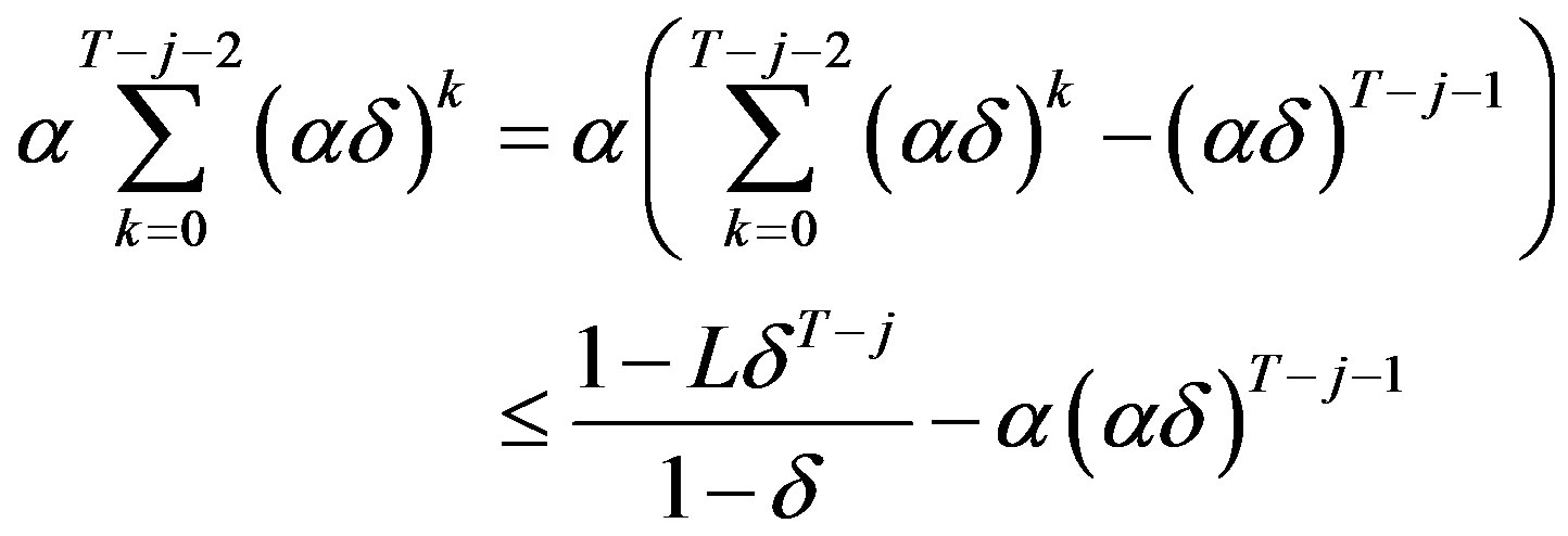
In the above, the inequality is given by the assumption (9). It is left to show that

.

This is true because:

which is true by the assumption that

Case 2—If: Since

is true for all i, condition (7) is strictly met, in particular, for all. QED.

We state and prove the following lemma, which is useful for the proof of Theorem 1.

Lemma 3:

Let and let denote the unique solution to

.

a).

b) if and only if, and if and only if.

c) and.

d) If then, and.

e) If then,

and

for.

Proof of Lemma 3:

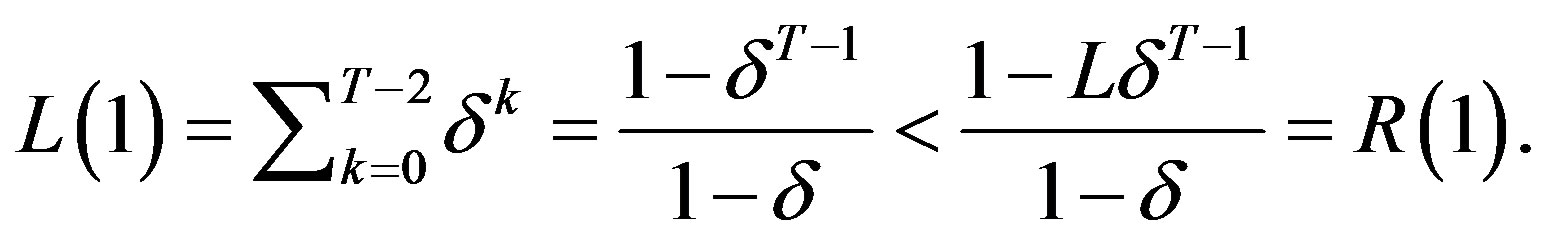
a) We start by showing that uniquely exists. Let

and let

and notice that by definition. Since, , L is strictly increasing, , , and R is strictly decreasing, a unique solution exists to the problem denoted by. Now, because

Finally, because

b) By (7), if and only if

if and only if. if and only if (7) is not satisfied for. Thus, if and only if

c) For any, if and only if

(10)

which holds true for all by Lemma 2 and the definition of. The second statement of c follows from

where the last inequality follows from condition (7).

d) By Lemma 2, when the inequalities in the proof of Part c are strict inequalities.

e) Since we have by Part a that.

Thus, and therefore. The second statement follows directly the inverting the inequality in (10) and the consequent derivations. Finally,

where the inequality results from and. QED.

Proof of Theorem 1:

The proof of the theorem is by backwards induction. Assume now that we are at period. We inductively assume that the optimal investment policy is given by:

Notice, in particular, that this assumption holds true for periods and. We will have to show the optimal investment policy in the ith period is given by

(11)

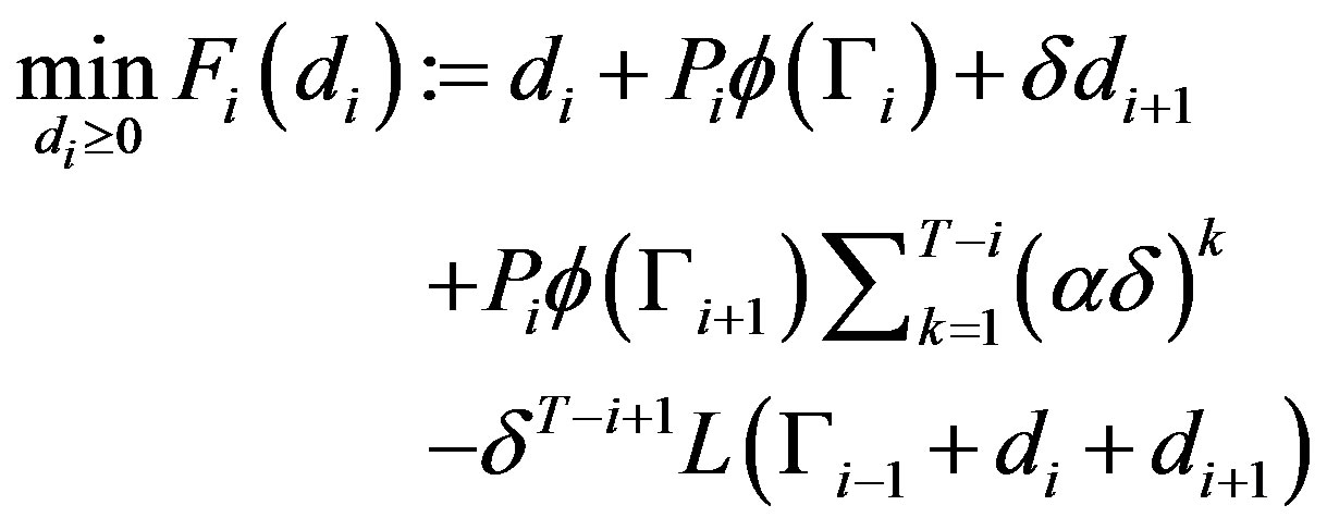
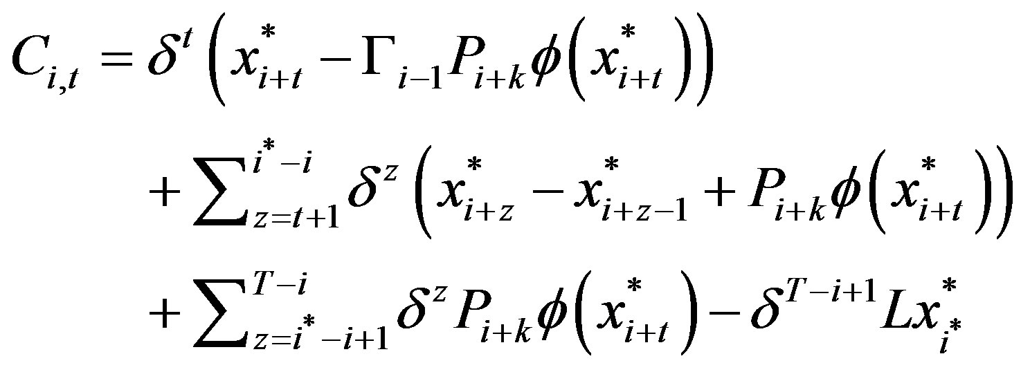
The firm’s problem at period i is to minimize its total expected amortized costs, given by

(12)

Case 1:

When, by Lemma 3c-d we have that for all,. Recall, by assumption,

and therefore, 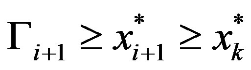for all. Consequently, our assumptions on future investment imply that and for all. We can therefore rewrite the firm’s problem, (12), as following

If we have that andconversely, if then. Thus,

(13)

where

.

We proceed to examine two separate cases:

Case 1a: We now assume that and therefore for all. The firm’s problem, (13), is therefore. First order condition is given by

.

Since, we conclude that

as in (11).

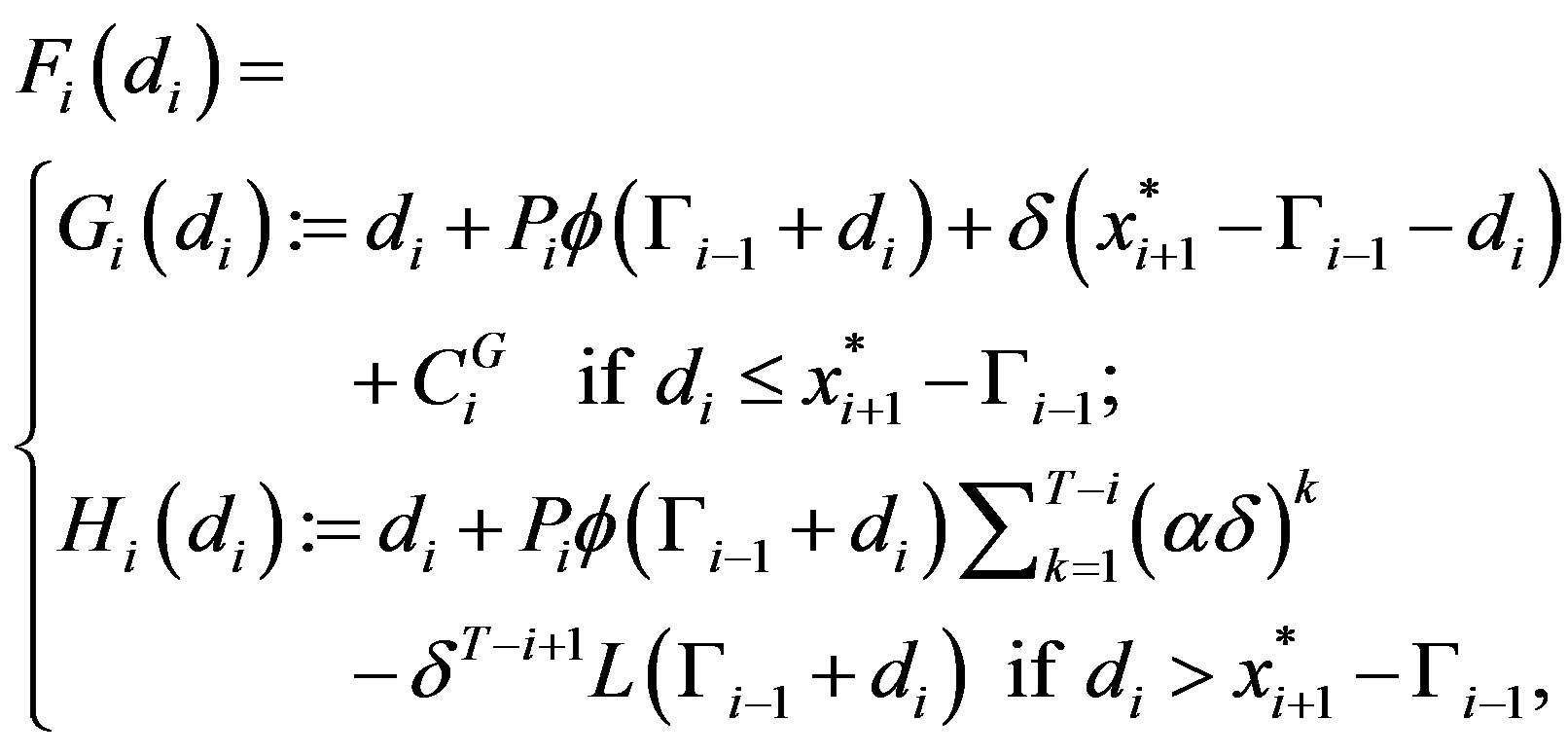
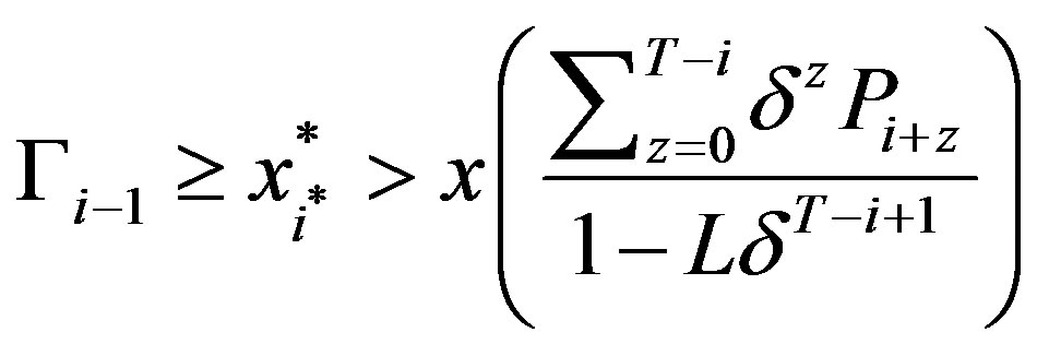
Case 1b: Assume now that. Since, by Lemma 3c-d, and showing (11) requires showing that. The firm’s problem(13), is3

(14)

Since, we can apply Lemma 1 to determine that the minimum of (14) on is.

By Lemma 3c-d,. Hence, we can apply Lemma 1 to determine that the minimum of (14) on the line segment is. Finally, since

we have that the optimal solution is. This concludes the derivation of theinduction argument for Case 1.

Case 2:

The key fact in the proof of Case 1 is that future threshold levels are non-increasing in time. Now, however, we have by Lemma 3 that the threshold levels are increasing until and non-increasing thereafter. In the non-increasing region, i.e. for all similarly to the case where we have that optimal investment is zero and that the reliability equals the maximal threshold.

Observe. By the induction assumption,

. If then it can be easily shown that the induction assumption implies that, where the inequality is replaced with equality if is sufficiently low. Repeating this analysis using the induction assumption and the definition of we produce the following rules:

If then:

If

for any, then:

Finally, if then:

;

for all. Consequently, the firm’s problem, (12), has the form:

where

, are independent of. In the above, we use the convention that if then.

We now consider three cases:

Case 2a.: The firm’s problem is given by:

(15)

Considering Lemma 1, the optimal solution of (15) is

.

Since, by Lemma 3e,

where the inequality can be shown by iteratively applying the second part of Lemma 3e. Thus,

and therefore the optimal solution is. Since, can be written as in (11).

Case 2b.: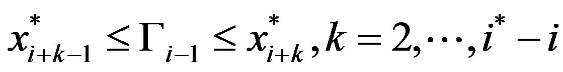

The firm’s problem is given by:

(16)

By Lemma 1, for any the optimal solution of

is.

Since,

for all, we can iteratively improve the solution by shifting from the region

to

and so forth until

and then to. Hence, the solution to (16) must lie on the segment. Employing Lemma 1, the solution to

is.

By Lemma 3e,

and therefore we have that

.

Thus, the optimal solution,. Since, can be written as in (11).

Case 2c.:

The firm’s problem is given by:

(17)

Using the same arguments as in Case 2b we have that the optimal solution to (17) is on the line segment. By Lemma 1 the solution to

is.

Since

the optimal solution is as in (11). QED.

The proof of Proposition 2 follows directly from Theorem 1 and the definition of condition (7) and is omitted.

The proofs of Proposition 3 and Theorem 2 follow from Lemma 3 and the discussion proceeding Theorem 2 and are omitted.

Proposition 4

a) If then clearly is non-decreasing. Assume, therefore, that and notice that this implies by Lemma 3a-b that. We now need to show that if for some pair condition (7) is not satisfied then it is not satisfied for, too. Suppose, therefore that

(18)

We need to show now that

.

In the above, the first inequality is given by the assumption (18) and the second inequality is true because

and.

b) Pick T. Let denote the solution of (8) when. By definition,

and

.

If

(19)

is true then by the same arguments of the proof of Lemma 3a we have that for any arbitrary T. It is therefore left to show (19).

.

The second equality in the above follows the definition of. To complete the proof we show that

.

This is true because

because.

c) For any T,

which is true since by Lemma 3c-d we have that for any period,

and. QED.

Proposition 5

The statements follow directly from the definition of and given by (7), Proposition 3, (8) and Theorem 1, respectively. QED.

Proposition 6

The statement for follows immediately by its definition. For, substituting in (8) we have

Thus,. QED.

NOTES

¹We discuss the special case in a separate section.

²See, for example, [2] for a description of the growth in recall costs in the automotive industry.

^*We slightly abuse notation for the convenience of having the point in both rows of (14). The problem (14) is nevertheless well defined because.

REFERENCES

- K. M. McDonald, “Recall the Recall,” Transportation Law Journal, Vol. 33, No. 3, 2006, pp. 253-292.
- K. M. McDonald, “Shifting out of Park: Moving Auto Safety from Recalls to Reason,” Lawyers & Judging Publishing, Tucson, 2006.
- A. Schiffauerova and V. Thomson, “A Review of Research on Cost of Quality Models and Best Practices,” International Journal of Quality & Reliability Management, Vol. 22, No. 6, 2006, pp. 647-669. http://dx.doi.org/10.1108/02656710610672470
- S. T. Foster, “An Examination of the Relationship between Conformance and Quality-Related Costs,” International Journal of Quality & Reliability Management, Vol. 13, No. 4, 1996, pp. 50-63. http://dx.doi.org/10.1108/02656719610114399
- A. V. Feigenbaum, “Total Quality Control,” 4th Edition, McGraw-Hill, New York, 2004.
- G. L. Gilardoni and E. A. Colosimo, “Optimal Maintenance Time for Repairable Systems,” Journal of Quality Technology, Vol. 39, No. 1, 2007, pp. 48-53.
- M. Freimer, D. Thomas and J. Tyworh, “The Value of Setup Cost Reduction and Process Improvement for the Economic Production Quantity Model with Defects,” European Journal of Operational Research, Vol. 173, No. 1, 2006, pp. 241-251. http://dx.doi.org/10.1016/j.ejor.2004.11.024
- J. Freiesleben, “Costs and Benefits of Inspection Systems and Optimal inspection Allocation for Uniform Defect Propensity,” International Journal of Quality & Reliability Management, Vol. 23, No. 5, 2006, pp. 547-563. http://dx.doi.org/10.1108/02656710610664604
- C. H. Fine and E. L. Porteus, “Dynamic Process Improvement,” Operations Research, Vol. 37, No. 4, 1989, pp. 580-591. http://dx.doi.org/10.1287/opre.37.4.580
- J. Voros, “The Dynamics of Price, Quality and Productivity Improvement Decisions,” European Journal of Operational Research, Vol. 170, No. 3, 2006, pp. 809-823. http://dx.doi.org/10.1016/j.ejor.2004.08.001
- G. Li and S. Rajagopalan, “The Impact of Quality on Learning,” Journal of Operations Management, Vol. 15, No. 3, 1997, pp. 181-191. http://dx.doi.org/10.1016/S0272-6963(97)00003-X
- G. Li and S. Rajagopalan, “Process Improvement, Quality, and Learning Effects,” Management Science, Vol. 44, No. 11, 1998, pp. 1517-1532. http://dx.doi.org/10.1287/mnsc.44.11.1517
- J. E. Carrillo and C. Gaimon, “Improving Manufacturing Performance through Process Change and Knowledge Creation,” Management Science, Vol. 46, No. 2, 2000, pp. 265-288. http://dx.doi.org/10.1287/mnsc.44.11.1517
- C. D. Ittner, “Exploratory Evidence on the Behavior of Quality Costs,” Operation Research, Vol. 44, No. 1, 1996, pp. 114-130. http://dx.doi.org/10.1287/opre.44.1.114
- C. D. Ittner, V. Nagar and M. V. Rajan, “Empirical Examination of Dynamic Quality-Based Learning Models,” Management Science, Vol. 47, No. 4, 2001, pp. 563-578. http://dx.doi.org/10.1287/mnsc.47.4.563.9831
- C. H. Fine, “A Quality Control Model with Learning Effects,” Operations Research, Vol. 36, No. 3, 1988, pp. 437-444. http://dx.doi.org/10.1287/opre.36.3.437