American Journal of Operations Research
Vol. 2 No. 3 (2012) , Article ID: 22413 , 12 pages DOI:10.4236/ajor.2012.23036
Phase Wise Supply Chain Model of EOQ with Normal Life Time for Queued Customers: A Computational Approach
Department of Mathematics & Statistics (Centre of Excellence on Advanced Computing), Dr. Ram Manohar Lohia Avadh University, Faizabad, India
Email: sant_x2003@yahoo.co.in, love_light59@yahoo.in
Received May 22, 2012; revised June 23, 2012; accepted July 4, 2012
Keywords: Supply Chain; Correlation; Normal Life Time; Dynamic Programming
ABSTRACT
In this paper, we mainly aim to compute the optimal inventory in the phase wise supply chain for queued customers in the interval of lower and upper bounds with particular life of the items. Important performance measures such as total optimal cost of the system and total expected delivery have also been computed by applying the dynamic programming and Drichlet theorem. Finally, numerical demonstration and sensitivity analysis have also been presented to gain the better perspective of the model.
1. Introduction
When an item is produced at any manufacturing centre, these items have to pass through different locations from the supply before reaching the items at final selling point. These locations are known as various phases of supply (these phases are not accessible by the end consumers or customers). For example, exploration of crude oils which is not readily available for the consumers and this has to pass though different phases of supply because of geographic inaccessibility due to terrain features such as mountains or lakes etc.; inability to purchase lease rightof-ways, and due to restricted wildlife areas. Similarly, other inventory items whose manufacturing can be easily accomplished because of easily available raw materials in that region but it has to go though different supply phases because of reasons as stated above before reaching the end consumers, for example, production of tea in India. Since these items have to under go various supply phases, their life times as well as their availability at particular time and at particular phase are subject to change due to time and climatic factors etc. In this situation analysis of optimum inventory resulting availability of inventory and their life times at any time is an interesting phenomenon to investigate by the researchers engaged in this field. Chen and Lin [1] employed the replenishment problem for deteriorating items with normally distributed shelf life, continuous time-varying demand, and shortages under the inflationary and time discount environment. Abdel [2] elaborated three mechanisms, namely food availability, food affordability and food accessibility. According to him in many other state-capitals, availability of food is not major constraint in the dynamics of the food system in supply chain. Shunji [3] illustrated briefly the concept of life time and the reliability of any operator which is working in various fields and the concept of availability is also correlated with the concept of reliability and its life time. Maike et al. [4] derived stationary distribution of joint queue length and inventory process in explicit product form for various M/M/1 systems with inventory under continuous review and different inventories management polices, and with lost sales.
Demand is Poisson, service times and lead times are exponentially distributed. These distributions used to calculate performance measures of the respective systems in case of infinite waiting room the key result is that the limiting distributions of the queue length process are the same as in the classical M/M/1/∞. Gerard et al. [5] discussed a queueing model in which two strategic servers based on their performance; the faster a server works, the more demand the server is allocated. The buyer’s objective is to minimize the average lead time received from servers. They found the considerable variation in the performance of allocation policies and concluded an effective procurement strategy for a buyer as long as the buyer explicitly accounts for the server’s strategic behaviour. Mishra and Yadav [6] dealt the profit optimization of a loss queueing system with the finite capacity and computed total expected cost (TEC), total expected revenue (TER) and total optimal profit (TOP) of the system. Mishra [7] discussed the cost analysis of G/M/C/K/N model including service rate and hyper geometric functions of other parameters in order to get optimal cost. Ravindran and Philips [8] solved a problem in oil transport technology in which the Black Gold Petroleum Company had found large deposits of oil on the North Slope of Alaska by considering the simple transportation networking and solving the problem for the optimum cost. Viswanathan and Mathur [9] considered a distribution system with a central warehouse and many retailers that stock a number of different products. Deterministic demand occurs at the retailers for each product. The warehouse acts as a break-bulk center and does not keep any inventory. The products are delivered from the warehouse to the retailers by vehicle routes used for the delivery, so as to minimize the long-run average inventtory and transportation costs. Iravani and Teo [10] considered the processing of M jobs in a flow shop with N stations in which only a single server is in charge of all stations. Their objective was to minimize the total setup and holding are cost, a class of easily implement able schedules is asymptotically optimal. Bellman [11] elaborated the theory of dynamic programming to solve the different type multi-echelon decision making problem of the management. We get fair motivation from Amitrajit [12], John [13], Mishra and Singh [14,15] and Sudhir et al. [16] in this field of investigation. Leonid and Luis [17] addressed that problem from a dynamic optimization of local decisions point of view, to ensure a global optimum for the supply chain performance. This is done under the frameworks of Collective Intelligence (COIN) theory and Multi-Agent Systems (MAS). By COIN, a large MAS where there is no centralized control and communication, but also, where there is a global task to complete the global supply chain network optimization. The proposed model focuses on the interactions at local and global levels between agents in order to improve the overall supply chain business process behavior. Besides, collective learning consists of adapting the local behavior of each agent (micro-learning) to the optimization of the behavior globally (macro-learning). Carrying cost which represents a large chunk of a company’s total supply chain costs so it has prominent role in the supply chain management. Inventory carrying costs are expressed as a percentage of the average dollar value of inventory over a fixed period usually a year. As a rule of thumb, inventtory carrying cost is 25% of a company’s average inventtory investment, but when you tally up all the relevant carrying costs, it can run as high as 40% or more. A while back a client asked me just how much it was costing him to carry inventory. I get this question all the time, and my answer is always the same: a company’s inventory carrying cost is, on average, 25% of its annual on hand inventory investment. From a financial point of view, understanding and managing inventory carrying cost will have an impact on your company’s operating income. It will also help you balance your operating expense with inventory levels. In operations, when purchasing and inventory control staff replenish an item, they ask themselves two basic questions: how much should we order, and when these aren’t trivial matters. Order more frequently, and your order cost increases while carrying costs decrease; less frequently, and you trade off lower order costs with a larger average inventtory. The most efficient way to figure out “how much” is to use the economic order quantity model. This model minimizes the total variable costs required to order and hold inventory. Inventory ordering cost, also known as purchasing cost or set-up cost, includes the clerical work required to prepare, release, monitor, and receive orders. In manufacturing, inventory ordering cost includes production scheduling time, machine set-up time, and inspection. Shaul et al. [18] illustrated an EOQ-type inventory problem where the demand rate is a function of the inventory level. It has been noted by marketing researchers and practitioners that an increase in a product’s shelf space usually has a positive impact on the sales of the product. In such a case, the demand rate is no longer a constant, but it depends on the amount of on-hand inventory. Erel [19] exulted the sensitivity of the basic economic order quantity (EOQ) model to continuous purchase price. The phenomenon of continuous price changes exists in several countries and it is not likely to improve. Wu and Low [20] exulted that the currently available economic order quantity-just-in-time (EOQ-JIT) cost indifference point models suggest that the JIT purchasing approach is always preferred to the EOQ approach when the JIT purchasing approach can capitalize on physical plant space reduction. It was found that these models did not empirically study the capability of an inventory facility to hold the EOQ-JIT cost indifference point’s amount of inventory. In addition, some important cost components under the inventory management systems were ignored by the models, for example, the out-of-stock costs and the impact of inventory policy on product quality, production flexibility. By developing the JIT purchasing threshold value (JPTV) models, it suggests that the advantages of JIT purchasing may have been overstated in theory. The JPTV models of this study overcome the two limitations of the existing EOQ-JIT cost indifference point models. Denis [21] used the information managerial techniques to solve the logistic problems which included the supply chain. Timo and Matti [22] examine the current state of inventory management in Finland by reviewing fifteen case studies made at the Lappeenranta University of Technology and several aspects of inventory management are considered by them. In greater detail, we have tried to answer questions such as: what is the role of inventory management in corporate planning, and how are inventory decisions made in manufacturing organizations? In addition particular attention is directed at the goal setting and performance measurement in inventory management. We have found out that important decisions concerning inventories are usually made at a low level in the organizational hierarchy with out any guidelines from top or middle management. Furthermore, companies lack accurate real time and suitably aggregate information of material flow and stock levels. This makes setting precise quantitative goals for inventory management difficult. Some companies have had financial pressure to decrease inventories and because of the lack of proper inventory control, this had led to both external and internal stock outs.
In the practice of phase wise supply chain model where customers are queued invite serious attention of professionals to compute the overall effectiveness of the model having normal life time of the inventory. Previously, this kind of model was not attempted for model had solution complexity because of use of multiple solution techniques. In this paper, performance measures related to the system has been analyzed and computed numerically. The total optimal cost of the system including inventory and queueing both systems, total optimal revenue and profit, optimal inventory in lower and upper bounds, and total expected waiting time of the customers to meet the inventory (total expected delivery time), have been discussed and finally computed. A set of multiple techniques such as dynamic programming, transportation networking and non-linear quadratic equations including an important Drichlet theorem have been used to analyze and compute performance measures of the system. Computing algorithm has been developed in order to compute performance measures. Observations have been drawn to discuss the sensitivity analysis related to various parameters of variations. The whole paper is organized in various sections such as introduction, description of the model, mathematical analysis, computing algorithm, numerical demonstration, observations and conclusion. Carrying costs are expressed as a percentage of the average dollar value of inventory over a fixed period usually a year. As a rule of thumb, inventory carrying cost is 25% of a company’s average inventory investment, but when you tally up all the relevant carrying costs, it can run as high as 40% or more. A while back a client asked me just how much it was costing him to carry inventory. I get this question all the time, and my answer is always the same: a company’s inventory carrying cost is, on average, 25% of its annual on hand inventory investment. From a financial point of view, understanding and managing inventory carrying cost will have an impact on your company’s operating income. It will also help you balance your operating expense with inventory levels. In operations, when purchasing and inventory control staff replenish an item, they ask themselves two basic questions: how much should we order, and when these aren’t trivial matters. Order more frequently, and your order cost increases while carrying costs decrease; less frequently, and you trade off lower order costs with a larger average inventory. The most efficient way to figure out “how much” is to use the economic order quantity model. This model minimizes the total variable costs required to order and hold inventtory. Inventory ordering cost, also known as purchasing cost or set-up cost, includes the clerical work required to prepare, release, monitor, and receive orders. In manufacturing, inventory ordering cost includes production scheduling time, machine set-up time, and inspection. Shaul et al. [18] illustrated an EOQ-type inventory problem where the demand rate is a function of the inventory level. It has been noted by marketing researchers and practitioners that an increase in a product’s shelf space usually has a positive impact on the sales of the product. In such a case, the demand rate is no longer a constant, but it depends on the amount of on-hand inventory. Erel [19] exulted the sensitivity of the basic economic order quantity (EOQ) model to continuous purchase price. The phenomenon of continuous price changes exists in several countries and it is not likely to improve. Wu and Low [20] exulted that the currently available economic order quantity-just-in-time (EOQ-JIT) cost indifference point models suggest that the JIT purchasing approach is always preferred to the EOQ approach when the JIT purchasing approach can capitalize on physical plant space reduction. It was found that these models did not empirically study the capability of an inventory facility to hold the EOQ-JIT cost indifference point’s amount of inventory. In addition, some important cost components under the inventory management systems were ignored by the models, for example, the out-of-stock costs and the impact of inventory policy on product quality, production flexibility. By developing the JIT purchasing threshold value (JPTV) models, it suggests that the advantages of JIT purchasing may have been overstated in theory. The JPTV models of this study overcome the two limitations of the existing EOQ-JIT cost indifference point models. Denis [21] used the information managerial techniques to solve the logistic problems which included the supply chain. Timo and Matti [22] examine the current state of inventory management in Finland by reviewing fifteen case studies made at the Lappeenranta University of Technology and several aspects of inventtory management are considered by them. In greater detail, we have tried to answer questions such as: what is the role of inventory management in corporate planning, and how are inventory decisions made in manufacturing organizations? In addition particular attention is directed at the goal setting and performance measurement in inventory management. We have found out that important decisions concerning inventories.
2. Description of the Model
Here, it is assumed that inventory items demanded in the market follow normal availability as well as normal lifetime.The reasons of choosing normal are twofold: it is one of the most important probability phenomena in the real world due to the classical central limit theorem, and it is also one of the most commonly used lifetime distributions in reliability contexts and Moreover, uncertainties inherent in customer demands make it difficult for supply chains to achieve just-in-time inventory replenishment, resulting in loosing sales opportunities or keeping excessive chain-wide inventories. Here, supply chain consists of one supplier and multiple retailers. The inventory-control parameters of the supplier and retailers are lead time and stocks. Customer-demand pattern is supposed to be proportional to the arrival of the customers at selling point which follows Poisson distribution.
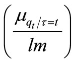
Also supply chain of items is considered from firm to the selling point of inventory items and supply time of the inventory items is exponential distribution to fulfill demand and interarrival time of demand follows exponential distribution at different phases. This shows that supply of inventory initially passes through different channels, and from each channel it passes through different phases to reach the selling points. Further, it is assumed that l is the numbers of channels and m is the partial integral quantity of the inventory available at one channel, is required at the selling point. Hence, partial amount of availability of items, at a selling point is f = lm. The partial quantity which is to reach selling point (last phase) of the average available quantity at the firm is given by  .
.
This average availability of inventory  rolls through all the locations (phases) in one chain of supply. This will be the average availability at the selling point (last phase) and customers (consumers) come at the selling point to get inventory with rate λ and follow Poisson Probability Distribution. At least
  amount is supplied by one phase to another phase till last phase (selling point). Since arrival of consumers at selling point, with rate λ follows Poisson distribution and service rate μ at selling point follow exponential distribution. Assuming that supply rate of inventory is R, inter supply time of inventory is also follow exponential distribution. Due to aforesaid assumptions consumers have to wait in queue in front of the selling point to get inventory items.
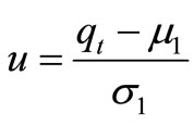
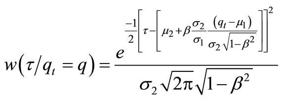
The following notations have been used throughout the paper qt = Available quantity at time t such that τ = Lifetime of inventory item such that
 μ1 = Mean of available quantityμ2 = Mean of lifetimeσ1 = Standard deviation of available quantityσ2 = Standard deviation of lifetime Here,<
  = Average available quantity of given lifetime τ = tβ = Correlation coefficient between availability and lifetime of inventory items,
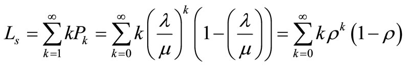
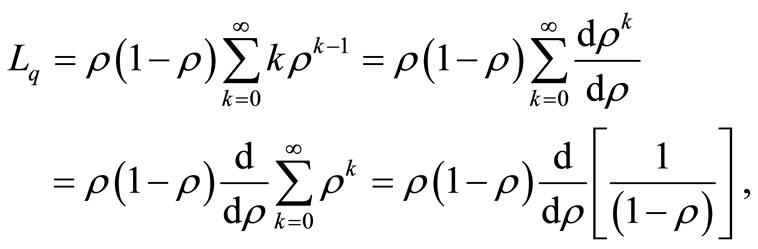
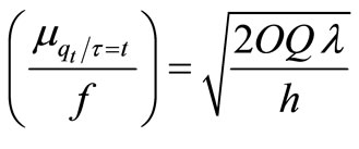
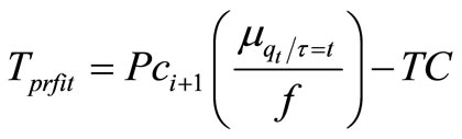
  = Partial amount of availability of itemsat a selling point, where f shows a positive integral quantity which is chosen by a selling point as per its requirement and this amount passes through n phasesh = Holding cost per unit time per unit quantity at each phasePC0 = Cost of raw material invested by ProducerPCn = Purchasing cost per unit quantity at the nth phaser% = Profit earned by each seller at every phaseLq = Waiting length of customer to find service at selling point (at last phase)ω = Waiting cost per customer in queueoi = Ordering cost per order at ith phaseO = Total ordering cost per cycle of whole systemR = Quantity received per order i.e. supplied quantity per orderλ = Arrival rate of customer at last phaseμ = Service rate at last phase to serve customersQ = Average quantity demanded by per customersi = Setup cost of ith phaseTpi = Transportation cost from (i − 1)th phase to ith phase per shipmentT = Total lead time of inventory from producer to last seller. It is also assumed one cycle time.
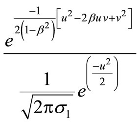
The n-phases are ascertained after solving supply chain networking; vide a sample networking in graph by using the concept of dynamic programming as discussed below in brief. Here, customers are arriving with Poisson rate λ at nth phase (a selling point for the customers) and receiving items with service rate μ. We here only discuss about the quantity which will reach at the last point of selling available for the consumers. The problem is solved by using dynamic programming if μ1 = 3σ1, μ2 = 3σ2 and a ≅ 0.9987, b ≅ 0.9987 and if μ1 = 2.5σ1, μ2 = 2.5σ2, a ≅ 0.9938, b ≅ 0.9938 In practice, if μ1 ≥ 2.5σ1, μ2 ≥ 2.5σ2 we assume a ≅ 1, b ≅ 1. For 0 < qt < ∞ and 0 < τ < ∞, where σ1 > 0, σ2 > 0 and ρ < 1. To study this joint probability, let us first show that parameter μ1 and μ2, σ1 and σ2 are the means and standard deviations of the two variables qt, τ. To begin with, we integrate on y from 0 to ∞ getting points so, it appears like network of supply of inventory. In this network we have to search the shortest route of supply of items. To find out minimum transportation cost route in this network by using Dynamic Programming.
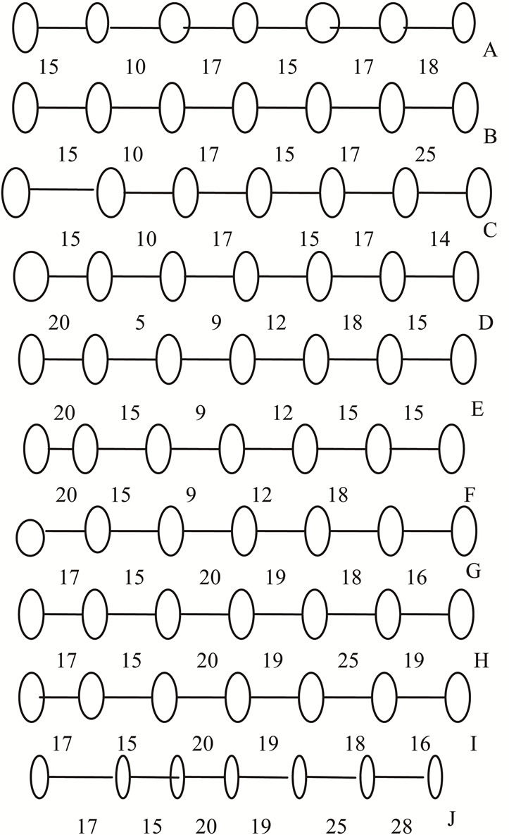
We present some sample networking to illustrate the model and which can further be generalized as per requirement of the supply chain we consider seven regions and seven stages to complete the chain from selling points to the point of origin (manufacturing point). Region and stages refer to various areas of operation and distance from the origin respectively. For example stage-I refers to last point of selling of customers level and region VII stands for a particular area if operation/ distribution related to end consumers. Further, region VII and stage I constitute the concept of phase (here last phase).
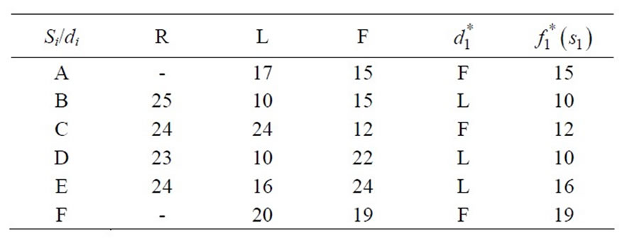
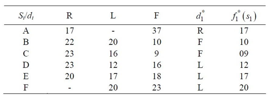
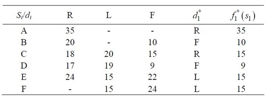
While solving, to find out shortest route (shortest chain of supply), we assume all the selling points under region-VII, and in stage-1, because we start from the selling point in the search of shortest route. After this we reach under region-VI, and in stage-2, the process of sorting is continue until we reach at the firm which is under region I and in stage-7. In each region, we assume that at least, there are three routes in three directions at each phase (location).These directions are Forward, Left and Right denoted by F, L, and R respectively. Taking decision at each Phase to choose the minimum value among F, L & R weights which is denoted by  After choosing minimum weighted path, we have to move in that direction. This process is continued until we have to reach in Region-I. This type of technique is also used in Graph Theory to find out the minimal weighed spanning tree. It is called Prim’s Algorithm. According to this algorithm we start from any vertex of graph and at that vertex we have to choose minimum length edge among the incidence edges. We traverse on it and reach at other vertex, again we employed the same procedures as afore said until we traverse at all vertices of graph.
Network of Supply Chain
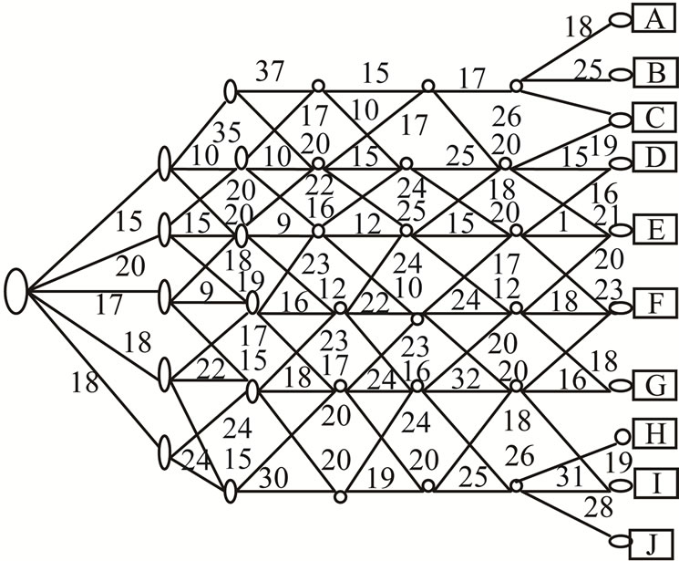
Minimum Transportation Route
 Stage 1 (REGION VII)
 Stage 2 (REGION VI)
 Stage 3 (REGION V)
 Stage 4 (REGION IV)
 Stage5 (REGION III)
 Stage 6 (REGION II)
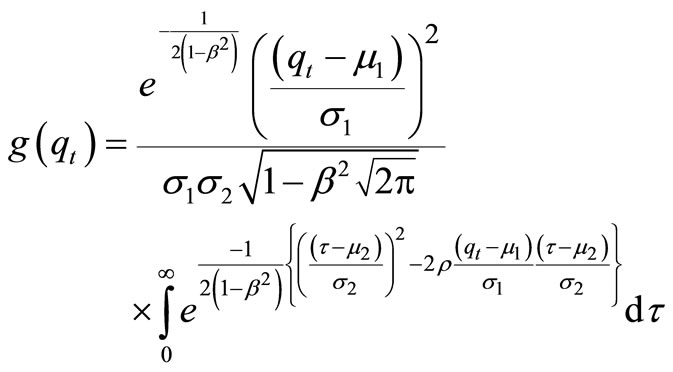
For marginal density of qt, then temporarily making the substitution 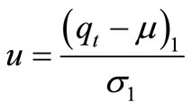
to simplify the notation and changing the variable of integration by letting
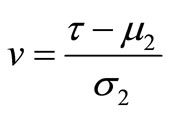 we obtained as

After completing the square by letting v2 – 2βuv = (v – βu)2 – β2u2 and collecting terms, this becomes (after identifying the quantity in parentheses as the normal density integral from 0 to +∞), we can equalize it to one. It consequently gives us
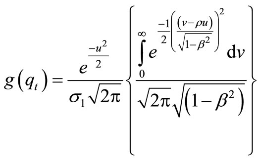

Accordance with definition and letting
 and
and 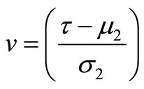
to simplify the notations, we get
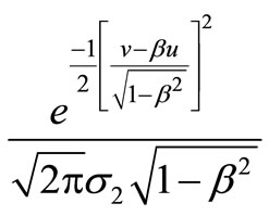
Then, expressing the term in original variables, we obtain
In this section, we have to make a simple model of route of transportation from firm to the selling points which are situated at different locations. Since there are number of routes from firm to sell.
Shortest Supply Chains (different phase wise supply routes)
Analogously, state k can enter only from state k − 1 since there is no state k + 1.
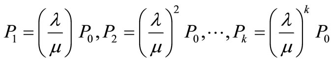
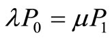
We now solve Equations (2)-(4) in terms of the stationary probability that the manager is idle, i.e. in terms of P0.
We get
 (5)
(5)
We can now use the fact that 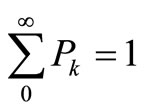 to solve for P0 explicitly. We get
 (6)
(6)
Let us assume that hi is holding cost per unit item at ith phase. Tpi is the transportation cost from i − 1 to ith phase. Pci is the purchasing cost of per unit item for ith phase. Si is the service cost per unit time to deliver service at ith Phase. It is assume that capacity of system is K. Thus the state space of the queue can be indexed by k, where k =1, 2, 3, ···, K.
That is when there are K customer in the system, Manager will not provide inventory to any more customers in certain time period.
So,
 (2)
(2)
where λ and μ are the parameters of the two exponential distributions, we get
 (3)
(3)
Finally for state k the rate equality principle gives me the following balance equation Using Equations (5) and (6), we get
 ; k =1, 2, 3, ···(7)

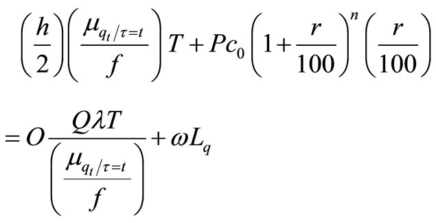
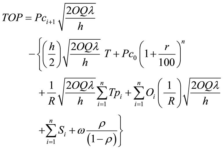
where We construct the total cost as
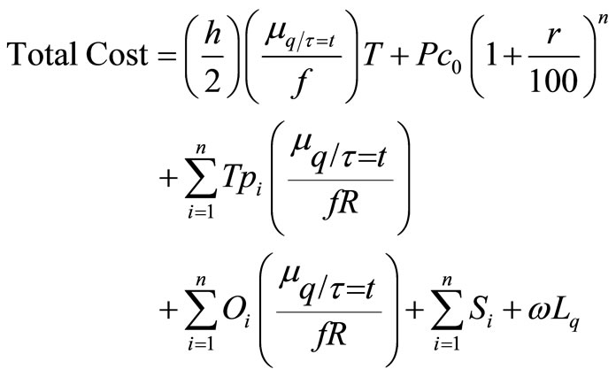 . (8)
. (8)
Here, we assume that demand of item is linear function of arrival i.e. D =Qλ where Q is aggregate quantity demanded by per customer, and  and inventory item is supplied from firm to the first whole seller of each channel and thereafter this it will pass through number of k-phases at each phase possesses

quantity but the last seller possesses approximate available quantity
where l is the number of channels and m is partial integral quantity of availability at one channel reached at last seller. Since both l, m are constant values so we consider lm = f. Hence
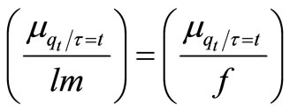 ;
;
Since this quantity will also roll through various phases of k. In case of inventory system, there exist mainly two types of contrary costs, one is carrying cost and another is ordering cost. In case of queuing system, it also has mainly two contrary costs. These are waiting cost and service cost. When we consider inventory system with queuing system then we get a supply chain system of inventory. In this supply chain system there are mainly four types of costs out of these costs, carrying cost and service costs are of the same nature, ordering cost and waiting cost, both are also of same. But sum of these pairs are contrary to each other. The intersection point of the contrary costs, which is found after sum, gives the optimal point for inventory as well as for optimal cost, it is given as below.
Carrying cost of items + Service cost (to serve items) = Ordering cost on inventory+ Waiting cost of customer in queue
Let us consider 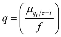 This implies that
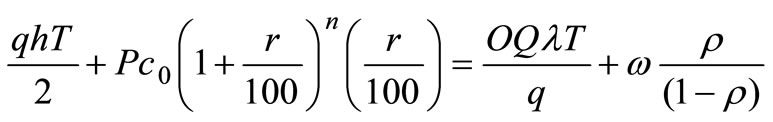
where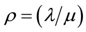 , λ is the arrival rate of customer and μ is service rate of inventory.
It finally turns out to yield

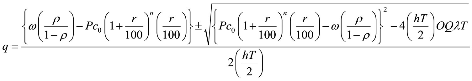
From above it is obvious that
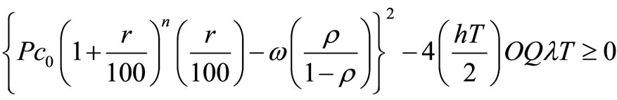
It further gives us
and finally.
According to the above inequality, we have to study about “q” in following two cases.
Case I
When
It implies that as
 ;
;
 ;
;
where 
Proof:
[Since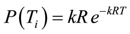 ].
].
Now applying Drichlet’s theorem of multiple integrals,
 ; k ≥ 0.

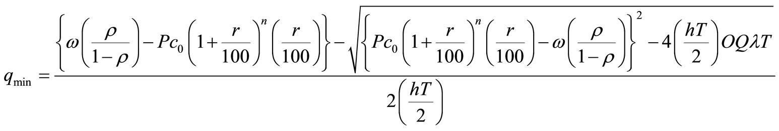
Case II
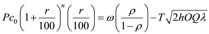

Substituting the value of qopt in Equation (1), we get total optimum cost
 ;
;
and so, 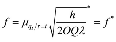
Let Oi is ordering cost invested by ith phase and ω is waiting cost per customer.

It finally gives total optimal cost as

We can also compute the total optimal profit as Total optimal profit for one seller = Total optimal Revenue – Total optimal cost;

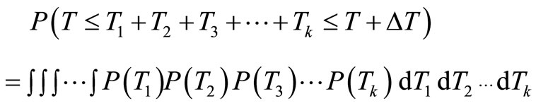
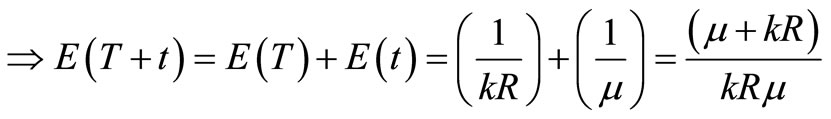
Thus we have delivery times T1, T2, T3, ···, Tk in k phases which are exponentially distributed variables with a common mean , and then T = T1 + T2 + T3 + ··· + Tk have the (Gamma) distribution with k phases and parameter R.
Hence expected lead time to deliver item from first to last phase is given as

Hence (Total expected time (for waiting inventory)
 ;
;
3. Computing Algorithm
Step 1: BeginStep 2: Input all the incident edges at one nodeStep3: Input all the parameters which are necessary to compute EOQ, TOC, TOP, and TEDTStep 4: Compute shortest edge from the incident edgesStep 5: Compute the minimum transportation cost from firm to selling pointStep 6: Compute the average availabilityStep 7: Compute average life-time of inventoryStep 8: Compute the optimal partial amountStep 9: Compute the maximum quantity which may available at selling pointStep 10: Compute the minimum quantity which may be demanded at selling pointStep 11: Compute the TOCStep12: Compute TOPStep 13: Compute TEDTStep 14: Stop.
Various numerical demonstrations are given on the basis of hypothetical data base system to study the variation of one parameter on the others.
4. Observations and Conclusions
The following important observations are drawn from the conducted research:
From Table 1, it is obvious that probability of quantity available in the store is independent of average life time, total optimal cost and also total expected delivery time.
Table 2, shows that when life-time of the inventory is increased then optimal partial amounts also increase.
From Table 3, we observe, that when correlation between life time and availability decreases then average availability, average life-time and optimal partial amount will also decrease.

Table 1. Probability of quantity available in terms of qt Verses TOC, TOP and TEDT Variables.
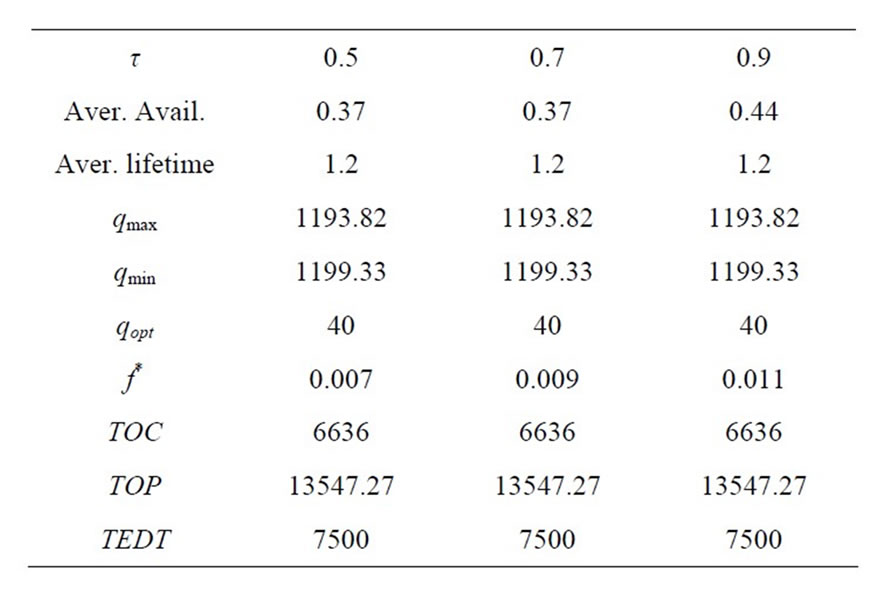
Table 2. Lifetime τ verses TOC, TOP and TEDT qt = 0.8,  , μτ = 0.3, σ1= 0.2, σ2 = 0.1, ρ = 0.7, Ch = 100, Cp = 200, r = 30, n = 10, ω = 90,000, t* = 3, μ = 50, λ = 40, R = 10, ρ = 0.7, Q = 40,
  , C0 = 50.
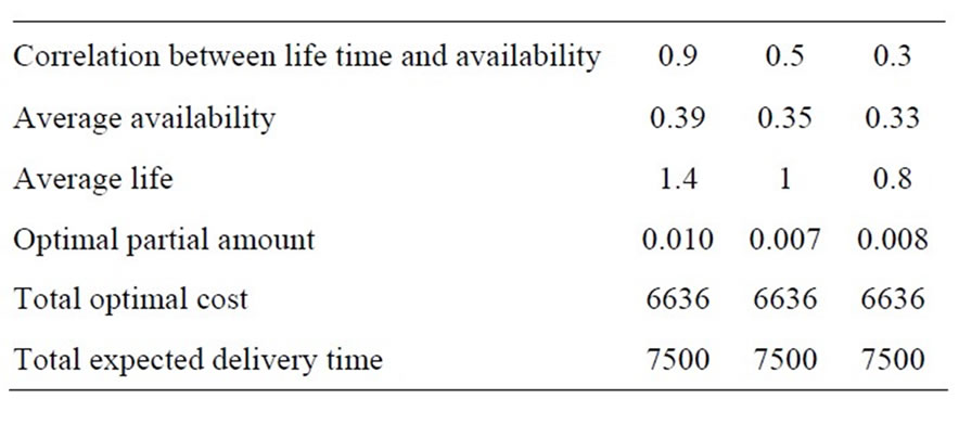
Table 3. Correlation coefficient r verses total optimal profit, total expected delivery time τ = 0.7,  , μτ = 0.3, σ1 = 0.2, σ2 = 0.1, Ch = 100, Cp = 200, r = 30, n = 10, μ = 50, λ = 40, R = 10, ω = 90,000, t* = 3, Q = 40,
  , C0 = 50.
It is also evident from Table 4 that when transportation cost is increased then total optimal cost as well as total optimal profit will also increase and average availability, optimal quantity and optimal partial amount will remain unaffected.
It is obvious from Table 5, that arrival rate of customers at selling point deceases then optimal quantity, total optimal cost and Total optimal profit will decrease but optimal partial amount will increase and other things remain unaltered.
Table 6 shows that when service rate at selling deceases then only total expected time will also decrease and another parameters remain unchanged.
We can conclude from Table 7, that when total demanded quantity at selling point increases then total optimal cost will increase but total optimal profit of the system remains constant.
In view of Table 8, we can say that when waiting time increases then maximum quantity as well as minimum
Table 4. Total cost verses total optimal cost, total optimal profit qt = 0.8, τ = 0.7,  , μτ = 0.3, σ1= 0.2, σ2 = 0.1, ρ = 0.7, Ch = 100, Cp = 200, r = 30, n = 10, μ = 50, λ = 40, R = 10, ω = 90000, ρ = 0.7, Q = 40,
  , C0 = 50.

Table 5. Total arrival rate λ verses total optimal cost, total optimal profit, TEDT qt = 0.8, τ = 0.7,  , μτ = 0.3, σ1 = 0.2, σ2 = 0.1, ρ = 0.7, Ch = 100, Cp = 200, r = 30, n = 10, μ = 50, R = 10, ω = 90,000, ρ = 0.7, Q = 40,
  , C0 = 50.

Table 6. Service rate μ verses total optimal cost, total optimal profit and TEDT qt = 0.8, τ = 0.7,  , μτ = 0.3, σ1 = 0.2, σ2 = 0.1, ρ = 0.7, Ch = 100, Cp = 200, r = 30, n = 10, λ = 40, R = 10, ω = 90000, ρ = 0.7, Q = 40,
  , C0 = 50.
quantity also increases. It means that range of quantity needed at selling point will increase. Table 9, justifies that when availability as well as optimal partial amount remains unchanged for insignificant changes in standard

Table 7. Quantity Q verses total optimal cost, total optimal profit and TEDT qt = 0.8, τ = 0.7,  , μτ = 0.3, σ1 = 0.2, σ2 = 0.1, ρ = 0.7, Ch = 100, Cp = 200, r = 30, n = 10, ω = 90,000, λ= 40, R = 10, ω = 90,000, Q = 40,
 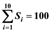 , C0 = 50.
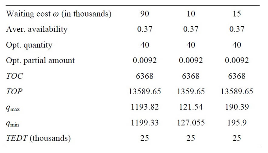
Table 8. Waiting cost ω verses total optimal cost, total optimal profit and TEDT, qmax, qmin qt = 0.8, τ = 0.7,  , μτ = 0.3, σ1 = 0.2, σ2 = 0.1, ρ = 0.7, Ch = 100, Cp = 200,
  , r = 30, n = 10, λ = 40, R = 10, ρ = 0.7, Q = 40, C0 = 50.

Table 9. Purchasing cost Cp verses total optimal cost, total optimal profit and TEDT, qmax, qmin qt = 0.8, τ = 0.7,  , μτ = 0.3, σ1 = 0.2, σ2 = 0.1, ρ = 0.7, Ch = 100, r = 30, n = 10, ω = 90,000, λ = 40, R = 10, ρ = 0.7, Q = 40,
  , C0 = 50.
deviations increase. In Table 10, as standard deviation increases the optimum partial amount decreases and optimal quantity.
From Table 11, it is obvious that when ordered quantity
Table 10. Standard deviation of life σ1, Standard deviation of availability σ2 verses optimal quantity, Optimal partial amount f* qt = 0.8, τ = 0.7,  , σ1 = 0.2, μτ = 0.3, σ2 = 0.1, ρ = 0.7, Ch = 100, Cp = 200, r = 30, n = 10, ω = 90,000, λ = 40, R = 10, ρ = 0.7, Q = 40,
  , C0 = 5.
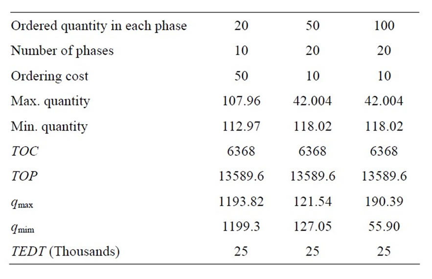
Table 11. Ordered qiamtotu R, m, C0 berses qmax, qmin and TOC, TOP, TEDT qt = 0.8, τ = 0.7,  , μτ = 0.3, σ1 = 0.2, σ2 = 0.1, ρ = 0.7, Ch = 100, Cp = 200, r = 30, ω = 90,000, λ = 40, R = 10, ρ = 0.7, Q = 40,
  , C0 = 5.
is increased then total optimal profit as well as total expected delivery time also increases but when number of phase increases then maximum quantity decreases as well as minimum quantity also decreases but total optimal cost as well as total optimal profit and total expected delivery time increase.
In this paper a fresh attempt has been made to compute the upper and lower bounds of the inventory items which can easily contribute to the management level of the organization. Decision on availability as well as life time of inventory can efficiently enhance the managerial decision makings, which are part of our paper deals with two systems simultaneously one is the supply chain of inventtories and another is the queueing system of consumers. This model is beneficial in the field of medicine supply chain as well as other expiry items whose life time follows the characteristics of the normal distribution. In practice for any organization it is very critical to find out the minimum transportation route for the optimum cost of the transportation. This part of problem is well-dwelt upon by us. Expected delivery time of inventory closely affect the decision makings related to supply chain management and system can be calibrated for better service to the customers in more-planned way.
REFERENCES
- J. M. Chen and C. S. Lin, “An Optimal Replenishment Model for Inventory Items with Normally Distributed Deterioration,” Production Planning and Control, Vol. 13, No. 5, 2002, pp. 470-480. Hdoi:10.1080/09537280210144446
- Abel, “Availability, Affordability and Accessibility of Food Khartoum,” GeoJournal, Vol. 34, No. 3, 2004, pp. 253- 255.
- S. Osaki, “Stochastic System Reliability Modeling,” Word Scientific Publishing, Singapore City, 1985.
- M. Schwarz, C. Sauer, H. Daduna, R. Kulik and R. Szekli, “M/M/1 Queueing Systems with Inventory,” Queueing System, Vol. 54, No. 1, 2006, pp. 55-78. Hdoi:10.1007/s11134-006-8710-5
- G. P. Cachon and F. Q. Zhang, “Obtaining Fast Service in a Queueing System via Performance-Based Allocation of Demand,” Management Science, Vol. 53, No. 3, 2007, pp. 408-420. Hdoi:10.1287/mnsc.1060.0636
- S. S. Mishra and D. K. Yadav, “Cost and Profit Analysis of M/Ek/1 Queueing System with Removable Service Station,” Bulgarian Journal of Applied Mathematical Sciences, Vol. 2, 2008, pp. 2777-2789.
- S. S. Mishra, “Computational Approach to the Cost Analysis of Dual Machine Interference Model with General Arrival Distribution,” PAMM, Vol. 7, No. 1, 2007, pp. 2060073-2060074. Hdoi:10.1002/pamm.200701034
- Ravindran and Philips, “O.R. Principle and Practice,” Solberg, New York, 2001.
- S. Viswanathan and K. Mathur, “Integrating Routing and Inventory Decisions in One-Warehouse Multiretailer Multiproduct Distribution Systems,” Management Science, Vol. 40, 1997, pp. 320-338
- S. M. R. Iravani and C. P. Teo, “Asymptotically Optimal Schedules for Single-Server Flow Shop Problems with Setup Costs and Times,” Operations Research Letters, Vol. 33, No. 4, 2005, pp.421-430. Hdoi:10.1016/j.orl.2004.08.007
- R. Bellman, “Some Problem in the Theory of Dynamic Programming,” Econometrica, Vol. 22, No. 1, 1954, pp. 37-48. Hdoi:10.2307/1909830
- A. A. Batabyal, “The Queueing Theoretic Approach to Groundwater Management,” Ecological Modeling, Vol. 85, 1996, pp. 219-227.
- J. E. Freund, “Mathematical Statistics,” Prentice Hall, Inc., New Jersey, 1992.
- S. S. Mishra and P. K. Singh, “Computational Approach to an Inventory Model with Ramp-Type Demand and Linear Deterioration,” International Journal of Operations Research, Vol. 15, No. 3, 2012, pp. 337-357.
- S. S. Mishra and P. K. Singh, “Computational Approach to EOQ Model with Power Form Stock-Dependent Demand and Cubic Deterioration,” American Journal of Operations Research, Vol. 1, 2011, pp. 5-13.
- S. J. Ryan Daniel, Chandrasekhar and Rajendran, “International Transactions in Operation Research,” Weily Inter Science, Vol. 12, 2005, pp. 101-127.
- L. Sheremetov and L. Rocha-Mier, “Supply Chain Network Optimization Based on Collective-Intelligence and Agent Technologies,” Human Systems Management, Vol. 27, 2008, pp. 31-47.
- K. Shaul, Bar-Lev, P. Mahmut and D. Perry, “On the EOQ Model with Inventory-Level-Dependent Demand Rate and Random Yield,” Operation Research, Vol. 6, 1994, pp. 167-176.
- E. Erel, “The Effect of Continuous Price Change in the EOQ,” Omega, Vol. 20, 2002, pp. 523-527. Hdoi:10.1016/0305-0483(92)90026-4
- M. Wu and L. S. Pheng, “Modeling Just-in-Time Purchasing in the Ready Mixed Concrete Industry,” International Journal of Production Economic, Vol. 107, 2007, pp. 190-201.
- D. R. Towill, “Logistics Information Management,” MCB UP Ltd., Vol. 9, 1996, pp. 41-53.
- T. Pirttilä and V.-M. Virolainen, “An Overview of the State and Problems of Inventory Management in Finland,” International Journal of Production Economics, Vol. 26, 1992, pp. 17-220.