Open Journal of Earthquake Research, 2013, 2, 75-83
Published Online November 2013 (http://www.scirp.org/journal/ojer)
http://dx.doi.org/10.4236/ojer.2013.24008
Open Access OJER
Strain Energy Release from the 2011 9.0 Mw Tōhoku
Earthquake, Japan
Kenneth M. Cruikshank, Curt D. Peterson
Department of Geology, Portland State University, Portland, USA
Received September 15, 2013; revised October 17, 2013; accepted October 31, 2013
Copyright © 2013 Kenneth M. Cruikshank, Curt D. Peterson. This is an open access article distributed under the Creative Commons
Attribution License, which permits unrestricted use, distribution, and reproduction in any medium, provided the original work is
properly cited.
ABSTRACT
The purpose of this paper is to compare the strain energy released due to elastic rebound of the crust from the tragic
2011 9.0 Mw Tōhoku earthquake in Japan with the observed radiated seismic energy. The strain energy was calculated
by analyzing coseismic displacements of 1024 GPS stations of the Japanese GEONET network. The value of energy
released from the analysis is 1.75 × 1017 J, which is of the same order of magnitude as the USGS-observed radiated
seismic energy of 1.9 × 1017 Nm (J). The strain energy method is independent of seismic methods for determining the
energy released during a large earthquake. The analysis shows that although the energy release is concentrated in the
epicentral region, about 12% of the total energy was released throughout the Japanese islands at distances greater than
500 km west of the epicenter. Our results also show that outside the epicentral region, the strain-energy was concen-
trated along known tectonic zones throughout Japan.
Keywords: Japan; Earthquake; Crustal Strain; GPS; Radiated Energy
1. Introduction
Reid’s [1] elastic rebound theory indicates that an under-
standing of the pattern and magnitude of strain in the
loading phase of the earthquake cycle is important for
evaluating the seismic risk in an area. Some insights into
the strain patterns in the loading phase can be gained by
examining the pattern of strain in the unloading or ear-
thquake phase. Measurements of tectonic strain release
during the 2011 Tōhoku earthquake and tsunami [2] (Fi-
gure 1) provide important insights into the mechanisms
of subduction zone earthquakes. These relations should
be of use in other subduction zones where modern strain
records might help to constrain predictions of earthquake
strain release and energy. To our knowledge, these are
the first wide-field comparisons of radiated energy and
observed strain energy reported for a subduction zone.
Analysis of strain energy provides a method for esti-
mating the total energy released without assuming a par-
ticular earthquake mechanism. For example, estimates of
the energy from an earthquake using either the Scalar
Moment or Observed Radiated Energy are often different
by 5 to 6 orders of magnitude, with the seismic moment
being substantially larger than the observed radiated en-
ergy [e.g., 3, Figure 12]. (Although, it should be noted
that the seismic moment is not a direct measure of the
energy released in an earthquake, so it will have a value
substantially different from the radiated energy [4]). Di-
rect measure of the strain between points on Earth’s sur-
face can be calculated from the relative displacement of
Global Positioning System (GPS) stations. GPS meas-
urements of crustal strain provide constraints on the dis-
tribution of energy release that are not directly available
from seismic stations alone.
In this paper we document the regional distribution of
coseismic strain in the upper plate from the 2011 Tōhoku
earthquake using length-changes between GPS stations
in the Japanese GPS network (GEONET, Figure 2). Our
estimate of the total strain-energy release, 1.75 × 1017 J,
is of the same order of magnitude as the observed radi-
ated seismic energy, 1.9 × 1017 J [2]. Our results also
show that a portion of the strain-energy was concentrated
along known tectonic zones throughout Japan (compare
Figures 1 and 3). These tectonic zones apparently served
as strain concentrators prior to the 2011 earthquake [5].
The distribution of strain release immediately following
the 2011 Tōhoku earthquake is generally consistent with
reported patterns of strain accumulation that have been
observed over the last 50 years [5,6].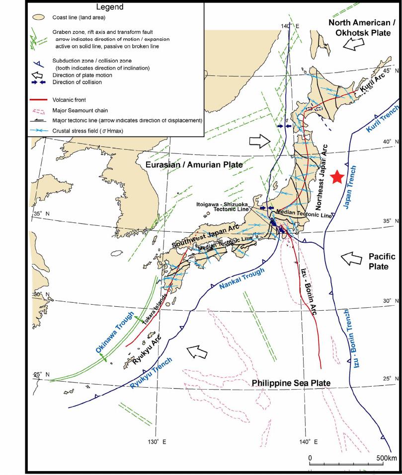

K. M. CRUIKSHANK, C. D. PETERSON 76
Figure 1. Map showing the current tectonic setting of Japan [Figure 6-2 from 7]. The 2011 epicenter, marked by a red star, is
located along the Japan Trench and the Northeast Japan Arc.
2. Background
The energy released in an earthquake is generally be-
lieved to come from the release of energy stored by the
elastic component of strain in the crust. This is the idea
expressed in Reid’s elastic rebound theory [1]:
“We know that the displacements which took place
near the fault-line occurred suddenly, and it is a matter
of much interest to determine what was the origin of the
forces which could act in this way. Gravity can not be
invoked as the direct cause, for the movements were
practically horizontal; the only other forces strong
enough to bring about such sudden displacement are
elastic forces. These forces could not have been brought
into play suddenly and have set up an elastic distortion;
but external forces must have produced an elastic strain
in the region about the fault-line, and the stresses this
induced were the forces which caused the sudden dis-
placements, or elastic rebounds, when the rupture oc-
curred”.
A similar mechanism is used to describe the release of
energy in phenomenon such as “rock bursts” in mines [8].
Open Access OJER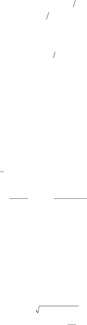

K. M. CRUIKSHANK, C. D. PETERSON 77
Here we consider the general energy balance for the
change in shape of an elastic material. We are not con-
cerned with any particular mechanism.
2.1. Energy Stored in Elastic Deformations
An elastic material is one where the original shape (the
unstrained state) will be restored after the forces causing
a change in shape (strain) are removed. An elastic mate-
rial can be thought of as a coiled spring, a spring that
resists both being shortened and lengthened. The resis-
tance of the spring to a change in length is the spring
constant; we take the value of the spring constant to be
the same for both shortening and extension, and the rela-
tionship force and change in length is described using
Hooke’s Law,
,
F
kL
where F is the force, k the “spring” constant, and ∆L the
change in length.
An elastic bar can be shortened by compressing it from
either end. The force does work in shortening the bar
(and so is using energy). Some of the energy may go into
heat generation or permanent shape changes but the re-
coverable energy which we are interested in will be
stored in the “springiness” of the elastic bar. Thus, the re-
sult of the change in length of the bar is net-energy
“storage” in the bar; this is the elastic strain energy. A
material will show elastic behavior as long as the length
change is small compared to the length of the bar, ge-
nerally less than 10−6 of the length of the bar.
In an elastic material the change in length is reversible
once the applied forces are removed (unloaded). When
the forces are removed from a bar it attempts to return to
its original length. The material many not completely
revert to its original geometry, since some of the poten-
tial energy has been converted to kinetic energy and heat.
If removal of the forces is a very slow process the kinetic
energy is negligible. If the removal of the forces is rapid
in addition to doing work to restore the materials shape a
portion of the stored potential energy will be converted to
kinetic energy which will be released as seismic waves.
Short term coseismic changes in length are an effect of
the elastic behavior of the rock, not the long-term defor-
mation, thus the elastic strain energy represents the
maximum potential energy that is available to be trans-
ferred to kinetic energy and observed as seismic waves.
In summary, the maximum amount of stored potential
elastic energy between two points in an elastic material is
proportional to change in distance between those two
points and the spring constant of the material. Using GPS
the change in distance between two points can be deter-
mined, which will then be proportional to the change in
elastic potential energy between the two points. This
change in elastic potential energy is the maximum
amount of energy that is available to be released as ki-
netic energy (i.e., seismic waves).
2.2. Strain and Strain Energy
Strain, ε, is the normalized change in length of a line
between two material points


StrainFinal LengthInitial LengthInitial Len
g
th


StrainChange in LengthInitialLength
or
1Strain Stretch


where
StretchFinal LengthInitialLength

Strain, ε, will be negative if the distance between two
points gets shorter (shortening), positive if the distance
increases (extension), and zero if it is unchanged. The
stretch (or stretch ratio), S, will be less than one for
shortening, greater than one for extension, and one for no
length change.
Over an area, strain (or stretch) provides a description
of deformation. This would consist of a series of strains
in different directions. Usually the strain is described
with two principle components. If we know the principle
components and their direction, we can describe the
strain in any arbitrary orientation.
Once the principle strains

123
,,


 are known, the
elastic strain energy is given by [8]:


2222
123123
12
2
eG
 




 (1)
where

21
E
Gv 

and

112
Ev
vv
  ,
where E is Young’s Modulus and v is Poisson’s Ratio.
In order to determine the principle strains we need the
strain in three different directions. The principle compo-
nent we end up with will represent some average strain
over the region enclosed by the three lines needed for the
solution.
GEONET stations were grouped into triangles, and
changes in position of the vertices were used to deter-
mine the magnitude of the principle strains (the solution
also gives the orientations, but that information is not
needed for this analysis). If we have three points, we can
define a triangle.
Consider a plane triangle, the Euclidian distance is:
22
Distance = dddENZ
2
1
base
d
Direction () = tand
E
N




Open Access OJER

K. M. CRUIKSHANK, C. D. PETERSON 78
where






d,d ,d
ABA BAB
EEENNNZZZ   .
If the direction is needed to be converted to an Azi-
muth ()

090;90
90360; 450.
if
if




 

 



Knowing the coordinates of A, B and C, the distances
between points can be determined. The direction of each
line element can also be determined.
Given displacements, dX and dY, the change of line
length can determined, allowing the strain of each line
segment to be determined. The displacement vector will
not always be parallel to the line segment, so we need to
get the component of the net displacement (imagine point
A is now fixed, so we look at the relative movement of
point B with respect to point A:
.
AB
AB
AB
NNN
EEE
Z
ZZ







This describes a net displacement vector with an ori-
entation of

1
tan ,
disp
E
N





and magnitude 22
dd dENZ
2
. The projection of
this vector into the direction of the line segment


b
ase

is accomplished by:
disp base
Angle π

 

222
= cosAngleLENZ  
to get the change in the vector direction of the line, or the
strain between the two stations
Since we are dealing with Geographic Coordinates, the
distance and line direction are determined using a modi-
fied Vincenty solution [9].
Evaluation of the strain energy (Equation (1)) requires
that the principal strains (εi) are known. Displacements of
GPS stations that comprise the 3 vertices of triangles in
the GEONET array provide sufficient information to
calculate the principal strains within the triangle [e.g., 10,
11]. The basic equations solved are (for irrotational strain,
[12]):
2
1
cos sinsincos
S
D
yx xy
YY XX
2




 



 





(2a)
where








.DxXyYxYyX  (2b)
S is stretch, and θ is the direction cosine for the line,
x
X

, yY

,
x
Y

, and yX are components
of the deformation gradient tensor [11,13]. Strain is
ii
1.S


 (2c)
Equations (2) are solved using displacements of three
GPS stations that make up the triangles shown in Figure
2; the evaluation of Equation (1) provides the strain en-
ergy density for the triangle. Using an average crustal
thickness, the total energy changes in the triangular prism
can be calculated.
From the principal strains, the average strain energy
density can be computed for a given area, assuming val-
ues of Young’s modulus (E) and Possion’s ratio (v). We
use Hanks and Kanamori [14] typical crustal values of 70
GPa and 0.25 respectively. In this paper we use an aver-
age crustal thickness of 30 km based on the USGS
CRUST 5.1 model [15] for the Japan region. Variations
in the value for average thickness do not significantly
change the results of estimated energy release (see Dis-
cussion).
2.3. Interpreting the “Total Energy Available”
Result
The results from Japan show that coseismic displace-
ments produce areas of shortening and areas of extension.
Since the elastic response makes no distinction between
energy released by the bar restoring to a longer or shorter
dimension, we take all of the areas to be generating po-
tential seismic energy.
Another extreme is to consider only areas extending to
be releasing stored energy, and area that are shortening to
be “absorbing” energy (although there is no a priori basis
for assuming this). If we do this, then the result is differ-
ent by 24% from the assumption for all areas releasing
energy. The order-of magnitude of the energy released is
the same (1017). We will use the all-cells releasing energy
figure, since that would represent the upper-limit of
available energy, although it is possible that about 12%
goes into “loading” other areas of the crust during the
earthquake.
3. Data and Methods
The Japanese nation-wide dense GPS network (GEONET,
Figure 2) has been in operation since 1996 [5]. In this
paper we only use displacements recorded in the 9
minutes following the March 2011 Tōhoku earthquake
(Figure 1). This allows us to exclude any movement
from aftershocks. The relative displacement of the GPS
stations represents the change in crustal strain. According
to Reid’s [1] elastic rebound theory the change in strain
represents stored elastic energy that is available to be
released as seismic waves.
Many of the 1024 stations in GEONET range from 20
Open Access OJER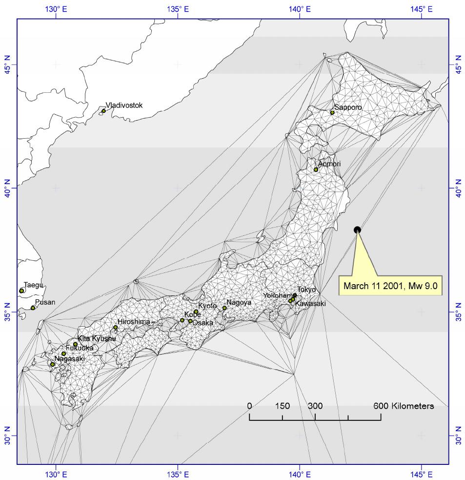

K. M. CRUIKSHANK, C. D. PETERSON
Open Access OJER
79
Figure 2. GPS stations that comprise the Japanese GEONET network and the Delauney Triangles that were formed using the
1024 GPS stations. Principal strains for each triangle are calculated, from which the strain energy density for each triangle is
computed.The location of the March 2011 Mw 9.0 earthquake is shown of the NE coast of Honshu.
to 40 km apart (Figure 2) and provide data coverage up
to 1500 km from the 2011epicenter. A network of 2393
triangles has been used to look at strain accumulation
over the last decade [e.g., 16]. Several stations are on
islands (Figure 2), thus strain in the oceanic crust to the
east of Japan can also be calculated, although at lower
resolution because of the increased distance between
GPS stations. We use the displacement of these stations
to calculate the energy released from stored elastic strain
as well as the distribution of energy release. This data
provides insight where strain energy was released or
stored following an earthquake, without the need to as-
sume a particular deformation model, e.g., displacement
discontinuities on a fault. GPS gives maps of coseismic
displacements that cannot be obtained from traditional
re-surveying of control networks that may take years
[e.g., 17,18] during which time additional displacements
may occur.

K. M. CRUIKSHANK, C. D. PETERSON 80
Data from GEONET was processed by the Advanced
Rapid Imaging and Analysis (ARIA) [19] team at
JPL/California Institute of Technology. Version 0.3 of
the processed data consisted of coseismic displacements
estimated from 5-minute interval kinematic solutions.
The coseismic displacements are the difference between
the solutions at 5:40 UTC and at 5:55 UTC. The earth-
quake occurred at 05:46 UTC, starting the 9 minute pe-
riod of strain measurements. Using this time frame
minimizes displacements from aftershocks and other
unrelated events. A search of the IRIS database (IRIS,
2011) for the region bounded by 128˚ to 146˚E, 29˚ to
46˚N and the GPS time frame found only the main shock
(Figure 2). The following steps were taken:
Stations were grouped to form non-overlapping train-
gles (Figure 2) [e.g., 20].
The initial latitude-longitude positions were used to
calculate the initial length (li) and direction (θi) for each
side in each triangle.
The displacements at each vertex in a triangle were
used to determine the final length of each side of the tri-
angle (Li) The triangles are an over-determined system.
Least-squares were used to solve for the maximum and
minimum principal strains (Equation (2)).
Multiplying the area of the triangle by the strain en-
ergy density (Equation (1)) gave the strain energy for a 1
m thick slab located within the triangle.
The energy per meter of thickness is multiplied by the
thickness of the crust (taken to be 30 km) to give the total
strain energy change in the vertical prism. The 30 km
crustal thickness was selected based on the USGS
CRUST 5.1 model [15].
4. Results
From the analysis of the ARIA data, the sum of the
energy per meter thickness of crust is 5.85 × 1012 J·m2.
Allowing for a crustal thickness of approximately 30 km,
the total energy is 1.75 × 1017 J. This value compares
well with the total radiated seismic energy (USGS, 2011)
of 1.9 × 1017 Nm (or J). Variations in elastic properties
and thickness of the crust would change our total strain
energy value, but by less than an order of magnitude.
Although the seismically-observed radiated energy is a
useful number, the strain-energy analysis shows the dis-
tribution of the sources and sinks of the energy (Figure 3)
without using a specific earthquake model, e.g., a dislo-
cation model. Some areas of the crust under Japan re-
leased energy while some areas may have stored energy.
This concept of differential loading and unloading has
generally been calculated using a specific model of the
faulting [e.g., 21]. From the change in strain the maxi-
mum available energy can be determined.
The variation in energy distribution can be seen by
looking at the “cumulative” energy as a function of dis-
tance from the trench axis (Figure 4).
Figure 3 shows the distribution of strain energy
sources and sinks throughout Japan. The green areas
represent triangles that increased in area, where the red
triangles represent areas of overall shortening.
5. Discussion
5.1. Surface Observations Related to the Whole
Crust
An assumption in GPS strain studies is that surface dis-
placements provide information about the elastic re-
sponse of the entire crustal material. Over the time-scale
of the coseismic energy release, a few minutes in dura-
tion, the crust can be regarded as a rigid elastic material.
By looking at the crustal response over a few minutes,
we do not have to consider the longer-term viscous be-
havior as observed at the year and decade time scales, of
the crustal material. Although, the changes in strain over
longer time intervals following an earthquake can pro-
vide important insights into longer-term crustal deforma-
tion and the partitioning of elastic and viscous behaviors,
it is not necessary in this study.
The assumption that the surface displacements are
representative of the strains throughout the crustal block
do appear to be valid because (1) the total energy calcu
lations agree with the independent radiated energy cal-
culation [2], and (2) the March 2011 Tōhoku earthquake
hypocenter is put at 30 km depth, which is near the re-
ported base of the upper-plate crust in the study area.
5.2. Influence of Thickness of Continental Crust
A 30 km crustal thickness was used to calculate the total
energy released of 1.75 × 1017 J from the strain energy
density of 5.85 × 1012 J per meter thickness of material.
The total energy released would range from 0.585 × 1017
J for a 10 km thick crust, to 2.93 × 1017 J for a 50 km
thick crust. The value changes by a factor of 5, but re-
tains the same order of magnitude as the observed radi-
ated energy. The value of 30 km was derived from the
USGS CRUST 5.1 model [15].
5.3. Pre-Earthquake Strain Measurements
Studies of accumulating strain patterns reflects deforma-
tion along several tectonic zones over long time periods
(earthquakes occurring during the measurement period),
whereas in this paper we only consider the effect of a
single earthquake along a single segment of a tectonic
zone, so reconciling the two patterns is difficult. How-
ever, our results indicate that several tectonic zones,
which were areas of increased strain accumulation in
previous studies, responded to the March 2011 Tōhoku
Open Access OJER

K. M. CRUIKSHANK, C. D. PETERSON
Open Access OJER
81
Figure 3. Strain energy density across the Japanese islands. White (land) and grey (oceanic) areas have a very low strain
energy density. Darker shading represents greater strain energies. Most of the total energy released is in the large triangles
around the epicenter. There is an area of high strain energy density at the southern margin of the rupture zone, just east of
Tokyo (Median Tectonic Line, Figure 1). About 5% of the total energy transfer is distributed along the southern coast of
Honshu and the West coast of Kyushu (compare with tectonic zones in Figure 1).
earthquake, when and where they became zones of con-
centrated energy release.
Harada & Simura [6] used three different first-order
triangulation surveys conducted over a 94 year range to
show the variability in the deformation in areas of Japan.
GEONET, which consisted of about 1000 stations at the
time, was used by Sagiya and others [16] to look at cur-
rent crustal deformation in Japan. They concluded that
most of the regions of large strain were associated with
tectonic boundaries and volcanoes. GEONET was also
used by Hasimoto and others [5] to investigate strain
accumulation from a slip-deficit model. All these studies
showed that regions of differing amounts of strain coin-
cided with known tectonic zones.
Strain energy release from the 2011 Tōhoku earth-
quake is shown in Figure 3; the denser-colored areas
show that the energy density was not uniform across the
study area. There is a band of higher strain energy density

K. M. CRUIKSHANK, C. D. PETERSON 82
Figure 4. Plot of energy released as a function of distance from the seismic front. The cumulative energy is the total energy
released by the entire area of GPS coverage. About 82% of the energy is released within 150 km West of the epicenter.
Another 12% is released 150 to 500 km west of the epicenter, and the remaining 6% is released more than 500 km west of the
epicenter. The jumps in energy released plot represent the concentrated energy release along tectonic zones.
running WSE-ENE along the southern end of the island
of Honshu, which corresponds to the Median Tec tonic
Line (Figure 1). The island of Kyushu, is another area of
increased strain energy density, which is at the intersec-
tion of the Ryukyu and SW Japan arcs. At the intersec-
tion of the Median and Itoigawa-Shizuoka tectonic lines,
located just East of Tokyo, is another area of increased
strain energy density. Interestingly, the Niigata-Kobe
Tectonic Zone, proposed by Sahiya and others [16], does
not appear to be a zone of high strain energy density.
Some of the variability in energy release can also be
seen by examining Figure 4. Eighty-two percent of the
energy is released within 150 km west of the epicenter.
Between 150 and 500 km west of the epicenter there was
rapid increases in total strain energy (a 6% and 4% rise).
These abrupt increases in energy release with distance
represent the crossing of the Median tectonic line just
east of Tokyo and the energy-dense area near Nagoya.
The gradual increase of total strain energy from 500 to
1100 km represents the energy released along the Median
Tectonic Line (Figure 1). There were smaller increases
of 1% - 2% increases approximately 1200 km west of the
epicenter, which represent the energy released in the is-
land of Kyushu.
Although the majority of the energy released in the
event was close to the epicenter approximately 12% of
the total energy was released 150 to 500 km away from
the epicenter (Figure 4). This 12% accounts for ap-
proximately 2.1 × 1016 J of energy, which is the observed
radiated seismic energy for a 7.5 Mw earthquake. This
landward release of energy could account for some of the
reported local strong shaking at substantial distances
from the epicenter.
In summary, pre-earthquake strain studies show non-
uniform strain accumulation with increased strain accu-
mulation along known tectonic boundaries. These areas
of increased strain accumulation showed high-strain en-
ergy densities of released elastic strain during the 2011
earthquake. The strain released in the 2011 9.0 Mw To-
hoku earthquake shows the same nature of differential
strain accumulation as seen by Harada & Simura [6] and
Hasimoto and others [5].
Open Access OJER

K. M. CRUIKSHANK, C. D. PETERSON 83
6. Conclusions
The 2011 9.0 Mw Tōhoku earthquake provides a unique
dataset of displacements over a large area during a
subduction zone earthquake. This study used 1204 GPS
stations, with an average station-to-station distance of 20
km. GPS data show coseismic displacements for the
earthquake using a 9-minute window of data following
the earthquake. Displacements from aftershocks are
excluded from the dataset, yielding the spatial variability
of co-sesimic displacements. Some conclusions are:
The amount of strain energy released is the same order
of magnitude as the observed radiated seismic energy.
About 12% if the total energy released (energy
equivalent to a Mw 7.5 earthquake) was released along
tectonic zones across the southern margin of Honshu.
Although energy release occurred throughout the Ja-
panese islands, it is concentrated in known tectonic
zones.
The pattern of different areas accumulating versus re-
leasing strain is similar to patterns of strain prior to the
2011 earthquake.
This paper has presented a method for calculating the
energy released in an earthquake that 1) is independent of
seismic energy methods, and 2) matches the seismically
observed radiated energy. This method could be applied
to areas that are currently accumulating strain to estimate
the amount of potential energy, and thus the magnitude
of an earthquake, that the area could generate during
megathrust fault rupture.
REFERENCES
[1] H. F. Reid, “The California Earthquake of April 18, 1906:
The Mechanics of the Earthquake,” The Carnegie Institu-
tion of Washington, Washington, D.C., 1908.
[2] USGS, US Geological Survey, Vol. 2011, 2011.
[3] H. Kanamori and E. E. Brodsky, “The Physics of Earth-
quakes,” Reports on Progress in Physics, Vol. 67, No. 8,
2004, pp. 1429-1496.
[4] S. Stein and M. Wysession, “An Introduction to Seismo-
logy, Earthquakes, and Earth Structure,” Blackwell, Mal-
den, 2003.
[5] C. Hashimoto, A. Noda, T. Sagiya and M. Matsu’ura,
“Interplate Seismogenic Zones along the Kuril-Japan
Trench Inferred from GPS Data Inversion,” Nature Geo-
science, Vol. 2, No. 2, 2009, pp. 141-144.
[6] T. Harada and M. Shimura, “Horizontal Deformation of
the Crust in Western Japan Revealed from First-Order
Triangulation Carried out Three Times,” Tectonophysics,
Vol. 52, No. 1-4, 1979, pp. 469-478.
[7] Nuclear Waste Management Organization of Japan,
“Evaluating Site Suitability for a HLW Repository (Sci-
entific Background and Practical Application of NUMO’s
Siting Factors),” Evaluating Site Suitability for a HLW
Repository (Scientific Background and Practical Applica-
tion of NUMO’s Siting Factors), Vol. NUMO-TR-04-04,
2004, pp. 29-39.
[8] J. C. Jaeger, N. G. W. Cook and R. W. Zimmerman,
“Fundamentals of Rock Mechanics,” Chapman and Hall,
London, 2007.
[9] T. Vincenty, “Direct and Inverse Solutions of Geodesics
on the Ellipsoid with Application of Nested Equations,”
Survey Review, Vol. 23, No. 176, 1975, pp. 88-93.
[10] F. C. Frank, “Deduction of Earth Strains from Survey
Data,” Bulletin of the Seismological Society of America,
Vol. 56, No. 1, 1966, pp. 35-43.
[11] L. E. Malvern, “Introduction to the Mechanics of Con-
tinuous Medium,” Prentice-Hall, Inc., Englewood Cliffs,
1969.
[12] K. M. Cruikshank, A. M. Johnson, R. W. Fleming and R.
Jones, “Winnetka Deformation Zone. Surface Expression
of Coactive Slip on a Blind Fault during the Northridge
Earthquake Sequence,” Open-File Report No. OF-96-698,
1996, p. 70.
[13] Y. C. Fung, “Foundations of Solid Mechanics,” Prentice-
Hall, Englewood Cliffs, 1965.
[14] T. Hanks and H. Kanamori, “A Moment Magnitude
Scale,” Journal of Geophysical Research, Vol. 84, No.
B5, 1979, pp. 2348-2350.
[15] W. D. Mooney, G. Laske and G. Masters, “CRUST5.1: A
Global Crustal Model at 5 × 5 Degrees,” Journal of Geo-
physical Research, Vol. 103, 1998, pp. 727-747.
[16] T. Sagiya, S. I. Miyazaki and T. Tada, “Continuous GPS
Array and Present-Day Crustal Deformation of Japan,”
Pure and Applied Geophysics, Vol. 157, No. 11-12, 2000,
pp. 2303-2322.
[17] G. Plafker, “Tectonics of the March 27, 1964 Alaska
Earthquake,” Professional Paper No. 543-I, 1969, p. 74.
[18] G. Plafker, “Alaskan Earthquake of 1964 and Chilean
Earthquake of 1960: Implications for Arc Tectonics,”
Journal of Geophysical Research, Vol. 77, No. 5, 1972,
pp. 901-925.
[19] ARIA, “Preliminary GPS Time Series Provided by the
ARIA (Advanced Rapid Imaging and Analysis) Team at
JPL and Caltech,” 2011.
ftp://sideshow.jpl.nasa.gov/pub/usrs/ARIA/
[20] B. Delaunay, “Sur la Sphère Vide,” Otdelenie Matemati-
cheskikh i Estestvennykh Nauk, Vol. 7, 1934, pp. 793-
800.
[21] G. C. P. King, R. S. Stein and J. Lin, “Static Stress Chan-
ges and the Triggering of Earthquakes,” Bulletin of the
Seismological Society of America, Vol. 84, No. 3, 1994,
pp. 935-953.
Open Access OJER