Applied Mathematics, 2011, 2, 254-257
doi:10.4236/am.2011.22029 Published Online February 2011 (http://www.SciRP.org/journal/am)
Generalized Abel Inversion Using Homotopy
Perturbation Method
Sunil Kumar, Om P. Singh, Sandeep Dixit
Department of Ap pl i e d Mat hematics, Institute of Technology, Banaras Hindu University, Varanasi, India
Received October 19, 2010; revised December 28, 2010; accepted January 3, 2011
Abstract
Many problems in physics like reconstruction of the radially distributed emissivity from the line-of-sight
projected intensity, the 3-D image reconstruction from cone beam projections in computerized tomography,
etc. lead naturally, in the case of radial symmetry, to the study of Abel’s type integral equation. Obtaining
the physically relevant quantity from the measured one requires, therefore the inversion of the Abel’s inte-
gral equation. The aim of this letter is to present a user friendly algorithm to invert generalized Abel integral
equation by using homotopy perturbation method. The stability of the algorithm is analysed. The validity and
applicability of this powerful technique is illustrated through various particular cases which demonstrate its
efficiency and simplicity in solving these types of integral equations.
Keywords: Generalized Abel Integral Equation, Homotopy Perturbation Method, Noise Term, Stability
1. Introduction
Since Abel formulated his integral equation [1] and pre-
sented its analytic solution, the equatio n has found appli-
cation in many branches of physical science. The earliest
application, due to Mach [2], arose in the study of com-
pressible flows around axially symmetric bodies. Usually,
physical quantities accessible to measurement are quite
often related to physically important but experimentally
inaccessible ones by Abel’s integral equation, [3-9]. Ob-
taining the physically relevant quantity from the meas-
ured one requires, therefore, the inversion of the Abel’s
integral equatio n, an d in case th e obj ect do es not h ave ra-
dial symmetry, it requires, in principal, the inversion of
Random transform.
We consider the following generalized Abel’s integral
equation

  0
,01, 0,
xyt dtg xx
xt

 

 (1)
where

g
xis the known function. The expression

x
t


 is called the kernel of the Abel’s integral equa-
tion or Abel kernel. An Abel’s integral equation belongs
to the class of Volterra equation of the first kind. If


g
x
is a continuously differentiable function, then the Abel’s
integral Equation (1 ) has a unique solution




1
0
sin ,
xgt
d
yx dt
dx xt





 [10] (2)
which is equivalent to
  

11
0
sin (0) .
xgt
g
yx dt
xxt















 (3)
Though, while the analytic solution to the Abel Equa-
tion (1) is given by (2), in practice we have only a point
wise approximation to g, so the inversion must be carried
out numerically. Since the integral transform (2) is equi-
valent to fractional differentiation of order 1


some
amplification of data noise is inevitable [11]. As the pro-
cess of estimating the so lution fun ction

,
y
x if the data
function


g
x is given approximately and only at a dis-
crete set of data points, is ill-posed since even very small,
high frequency errors in the measured

g
x, such as will
arise from experimental errors, photon counting noise and
noise in the electronics, might cause large errors in the
reconstructed solu tion


.
y
x This is due to the fact that
inversion formula (3) requires differentiating the meas-
ured data


g
x. In 1982, an analytic but derivative free
inversion formula was obtained by Deutsch and Benia-
miny [12] to avoid this problem. In addition, many nu-
merical inversion methods [13-21] have been developed
with varying degree of success with the inherent limita-

S. KUMAR ET AL.
255
tions of all measured data. Consequently, the direct use
of (2) and (3) are restricted and stable numerical methods
become important.
The aim of the present letter is to propo se an algorith m
to invert the Abel’s integral Equation (1) by using the
homotopy perturbation method (HPM). We construct a
convex homotopy by using HPM to obtain an iterative
solution to (1) and analyze the stability of the algorithm.
Some numerical examples are also presented to illustrate
the accuracy of the algorithm.
2. Method of Solution
In this method, using the homotopy technique of topol-
ogy, a homotopy is constructed with an embedding pa-
rameter


0,1 ,p which is considered as a “small para-
meter”. When the homotopy theory is coupled with per-
turbation theo ry it provide s a powerful mathematical tool.
The details of the method can be found in [22-24].
We constru c t th e following convex homotopy
 
  0
10,
xLt
pLxpdt gx
xt


 




 (4)
to develop a numerical inversion algorithm for the Abel
integral Equation (1), where the embedding parameter


0,1p can be consider as an expanding parameter
[23], to obtain
 
0
,
ii
i
LxpL x


 (5)
where,

,0,1,2,3,
i
Lx i are the functions to be de-
termined. We use the following iterative scheme to eva-
luate

i
Lx.
Substituting (5) in (4 ) and the equatin g the co efficients
of p with the same power, we get
 
 

 

 

01
01
1 221
0
2 332
0
1
10
:0,: ,
:,
:,
:.
x
x
xn
nnn
pLxpLx gx
Lt
pLx Lxdt
xt
Lt
pLx Lxdt
xt
Lt
pLx Lxdt
xt















 (6)
Hence the sol u t ion of Equati o n ( 1 ) is gi v en by
 
10
lim .
i
pi
yxLxL x



 (7)
Now, we consider the stability of the solution (7) to
small changes in data. That is we are interested in what
happens to y, when we replace


g
x by



g
xgx  ,
where


,
g
x  is unknown apart from some restriction
on its magnitude relative to

.
g
x For computational
convenience, we write
 
1.
g
xx   Subsequently,
the iterative scheme (6) becomes


 
 
 
0
11
221
0,
,
,
,
nnn
Lx
Lx gxx
Lx Lxx
Lx Lxx











(8)
where


n
Lx is given by (6) and
 



1
10
xn
nn
t
x
xdt
xt







, for n=2,3,4,
Thus, the new solut i o n

,
y
x
 is given by
 
0
lim .
n
i
ni
y
xLx
 

 (9)
The effect of the noise

1
x
 in the data deviates the
solution by
 

0
0
lim
lim ,
n
ii
ni
n
i
ni
yxyxyxL xL x
x


 
 

 






(10)
where


10.x


From (10), we conclude that
y

and
g

are con-
nected via the following generalized Abel integral equa-
tion


 
0
.
xyt dtg x
xt




 (11)
Thus, we have pro ved the fol lowing theorem
Theorem. The presence of a noise term


g
x  in the
observable data


g
x changes the solution


y
x by
an amount equivalent to the solution of the Abel integral
Equation (11) with input equal to the noise term


g
x 
itself.
As


g
x  is not known before hand, we take an up-
per bound for


g
x  . Let

01
sup ,
xgx


 then (11)
reduces to


 0
,
xyt dt
xt





 which can be readily solved.
3. Numerical Examples
The simplicity and accuracy of the proposed algorithm is
illustrated by the following numerical examples. We
compute the error


ˆ Exyx yx



, where


y
x
is the exact solution and

y
x is an approximate solu-
tion of the problem obtained by truncating equation (7).
Examples. To illustrate the method, we consider the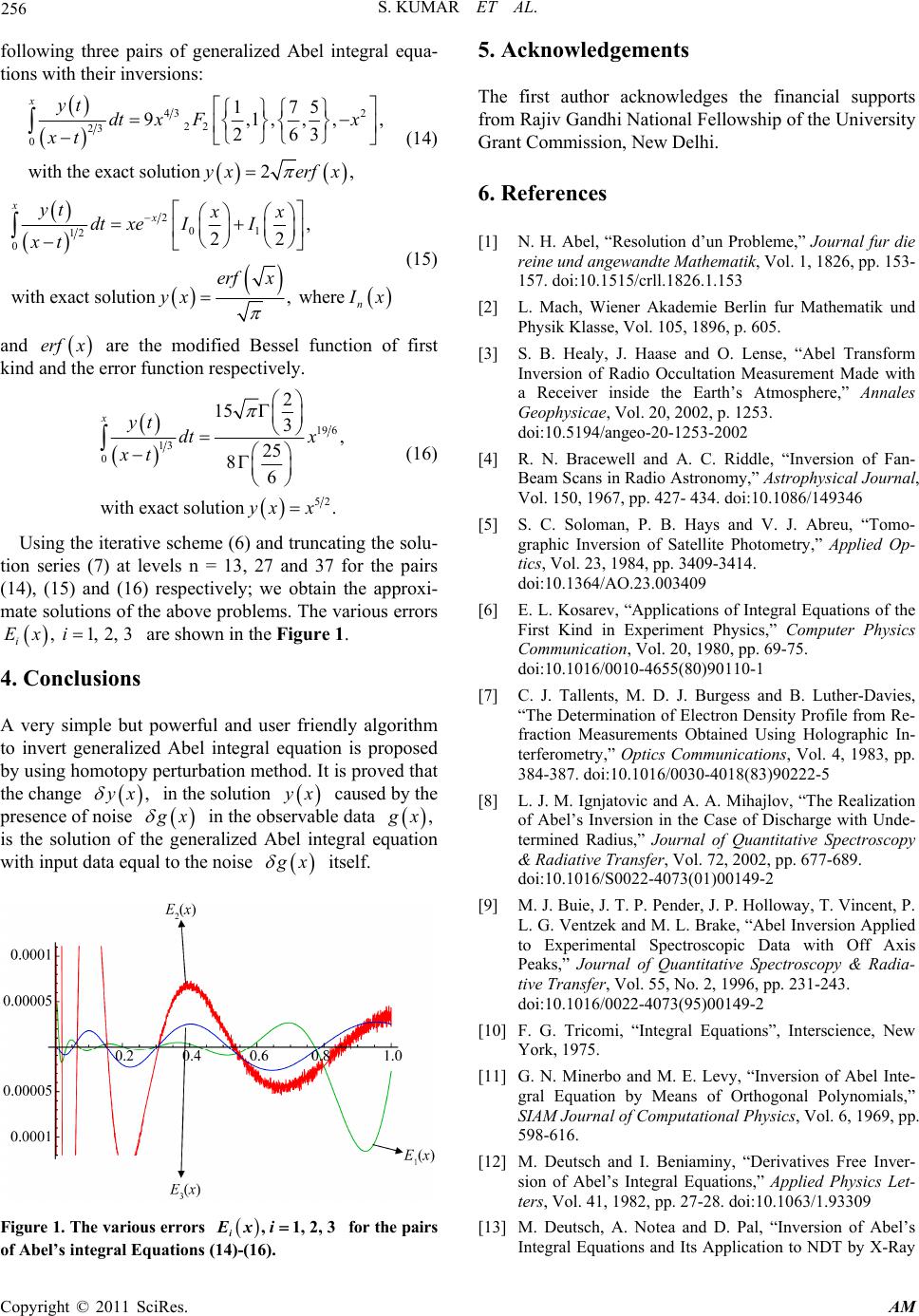

S. KUMAR ET AL.
256
following three pairs of generalized Abel integral equa-
tions with their inversions:


 
43 2
22
23
0
175
9,1,,,,
263
with the exact solution 2,
xyt dtx Fx
xt
yxerf x


 

 

  

 (14)





201
12
0
,
22
with exact solution , where
xx
n
yt xx
dt xeII
xt
erf x
yxI x


 

  
  


(15)
and

erfx are the modified Bessel function of first
kind and the error function respectively.



19 6
13
0
52
2
15 3,
25
86
with exact solution .
xyt dt x
xt
yx x








 (16)
Using the iterative scheme (6) and truncating the solu-
tion series (7) at levels n = 13, 27 and 37 for the pairs
(14), (15) and (16) respectively; we obtain the approxi-
mate solutions of the above prob lems. The various errors


,1,2,3
i
Ex i are shown in the Figure 1.
4. Conclusions
A very simple but powerful and user friendly algorithm
to invert generalized Abel integral equation is proposed
by using homotopy perturbation method. It is proved that
the change


,
y
x  in the solution


y
x caused by the
presence of noise


g
x  in the ob servab le data


,
g
x
is the solution of the generalized Abel integral equation
with input data equal to the noise

g
x 
itself.
Figure 1. The various errors


, 1,2,3
i
Exi for the pairs
of Abel’s integral Equations (14)-(16).
5. Acknowledgements
The first author acknowledges the financial supports
from Rajiv Gandhi National Fellowship of the University
Grant Commission, New Delhi.
6. References
[1] N. H. Abel, “Resolution d’un Probleme,” Journal fur die
reine und angewandte Mathematik, Vol. 1, 1826, pp. 153-
157. doi:10.1515/crll.1826.1.153
[2] L. Mach, Wiener Akademie Berlin fur Mathematik und
Physik Klasse, Vol. 105, 1896, p. 605.
[3] S. B. Healy, J. Haase and O. Lense, “Abel Transform
Inversion of Radio Occultation Measurement Made with
a Receiver inside the Earth’s Atmosphere,” Annales
Geophysicae, Vol. 20, 2002, p. 1253.
doi:10.5194/angeo-20-1253-2002
[4] R. N. Bracewell and A. C. Riddle, “Inversion of Fan-
Beam Scans in Radio Astronomy,” Astrophysical Journal,
Vol. 150, 1967, pp. 427- 434. doi:10.1086/149346
[5] S. C. Soloman, P. B. Hays and V. J. Abreu, “Tomo-
graphic Inversion of Satellite Photometry,” Applied Op-
tics, Vol. 23, 1984, pp. 3409-3414.
doi:10.1364/AO.23.003409
[6] E. L. Kosarev, “Applications of Integral Equations of the
First Kind in Experiment Physics,” Computer Physics
Communication, Vol. 20, 1980, pp. 69-75.
doi:10.1016/0010-4655(80)90110-1
[7] C. J. Tallents, M. D. J. Burgess and B. Luther-Davies,
“The Determination of Electron Density Profile from Re-
fraction Measurements Obtained Using Holographic In-
terferometry,” Optics Communications, Vol. 4, 1983, pp.
384-387. doi:10.1016/0030-4018(83)90222-5
[8] L. J. M. Ignjatovic and A. A. Mihajlov, “The Realization
of Abel’s Inversion in the Case of Discharge with Unde-
termined Radius,” Journal of Quantitative Spectroscopy
& Radiative Transfer, Vol. 72, 2002, pp. 677-689.
doi:10.1016/S0022-4073(01)00149-2
[9] M. J. Buie, J. T. P. Pender, J. P. Holloway, T. Vincent, P.
L. G. Ventzek and M. L. Brake, “Abel Inversion Applied
to Experimental Spectroscopic Data with Off Axis
Peaks,” Journal of Quantitative Spectroscopy & Radia-
tive Transfer, Vol. 55, No. 2, 1996, pp. 231-243.
doi:10.1016/0022-4073(95)00149-2
[10] F. G. Tricomi, “Integral Equations”, Interscience, New
York, 1975.
[11] G. N. Minerbo and M. E. Levy, “Inversion of Abel Inte-
gral Equation by Means of Orthogonal Polynomials,”
SIAM Journal of Computational Physics, Vol. 6, 1969, pp.
598-616.
[12] M. Deutsch and I. Beniaminy, “Derivatives Free Inver-
sion of Abel’s Integral Equations,” Applied Physics Let-
ters, Vol. 41, 1982, pp. 27-28. doi:10.1063/1.93309
[13] M. Deutsch, A. Notea and D. Pal, “Inversion of Abel’s
Integral Equations and Its Application to NDT by X-Ray

S. KUMAR ET AL.
257
Radiography,” NDT International, Vol. 23, No. 1, 1990,
pp. 32-38.
[14] J. P. Lanquart, “Error Attenuation in Abel Inversion,”
Journal of Computational Physics, Vol. 47, 1982, pp.
434-443. doi:10.1016/0021-9991(82)90092-4
[15] L. J. M. Ignjatovic and A. A. Mihajlov, “The Realization
of Abel’s Inversion in the Case of Discharge with Unde-
termined Radious,” Journal of Quantitative Spectroscopy
& Radiative Transfer, Vol. 72, 2002, pp. 677-689.
doi:10.1016/S0022-4073(01)00149-2
[16] V. K. Singh, R. K. Pandey and O. P. Singh, “New Stable
Numerical Solution of Singular Integral Equations of
Abel Type by Using Normalized Bernstein Polynomials,”
Applied Mathematical Sciences, Vol. 3, No. 5, 2009, pp.
241-255.
[17] O. P. Singh, V. K. Singh and R. K. Pandey, “New Stable
Numerical Inversion of Abel Integral Equation Using
Almost Bernstein Operational Matrix,” Journal of Quan-
titative Spectroscopy & Radiative Transfer, Vol. 111,
2010, pp. 245-252. doi:10.1016/j.jqsrt.2009.07.007
[18] I. Beniaminy and M. Deutsch, “Abel Stable High Accu-
racy Programme for the Inversion of Abel’s Integral
Equation,” Computer Physics Communication, Vol. 27,
1982, pp. 415-422. doi:10.1016/0010-4655(82)90102-3
[19] D. A. Murio, D. G. Hinestroza and C. E. Mejia, “New
Stable Numerical Inversion of Abel’s Integral Equation,”
Computers and Mathematics with Applications, Vol. 23,
No. 11, 1992, pp. 3-11.
doi:10.1016/0898-1221(92)90064-O
[20] S. Ma, H. Gao, L. Wu and G. Zhang, “Abel Inversion
Using Legendre Polynomials Approximations,” Journal
of Quantitative Spectroscopy & Radiative Transfer, Vol.
109, 2008, pp. 1745-1757.
doi:10.1016/j.jqsrt.2008.01.013
[21] S. Ma, H. Gao, G. Zhang and L. Wu, “Abel Inversion
Using Legendre Wavelet Expansion,” Journal of Quanti-
tative Spectroscopy & Radiative Transfer, Vol. 107, 2007,
pp. 61-71. doi:10.1016/j.jqsrt.2007.01.054
[22] J. H. He, “An Approximate Solution Technique Depend-
ing upon an Artificial Parameter,” Communications in
Nonlinear Science and Numerical Simulation, Vol. 3, No.
2, 1998, pp. 92-97. doi:10.1016/S1007-5704(98)90070-3
[23] J. H. He, “Homotopy Perturbation Technique,” Computer
Methods in Applied Mechanics and Engineering, Vol.
178, 1999, pp. 257-262.
doi:10.1016/S0045-7825(99)00018-3
[24] J. H. He, “A Review on Some Recently Developed
Nonlinear Analytical Technique,” International Journal
of Nonlinear Sciences and Numerical Simulation, Vol. 1,
No. 1, 2000, pp. 51-70.