Applied Mathematics, 2011, 2, 189-195
doi:10.4236/am.2011.22021 Published Online February 2011 (http://www.SciRP.org/journal/am)
On the Distribution of Type II Errors in
Hypothesis Testing
Skip Thompson
Department of Mathematics and Statistics, Radford University Radford, USA
Received October 16, 2010; revised November 26, 2010; accepted November 30, 2010
Abstract
When a statistical test of hypothesis for a population mean is performed, we are faced with the possibility of
committing a Type II error by not rejecting the null hypothesis when in fact the population mean has
changed. We consider this issue and quantify matters in a manner that differs a bit from what is commonly
done. In particular, we define the probability distribution function for Type II errors. We then explore some
interesting properties that we have not seen mentioned elsewhere for this probability distribution function.
Finally, we discuss several Maple procedures that can be used to perform various calculations using the dis-
tribution.
Keywords: Complementary Error Function, Hypothesis Testing, Power Curves, Power Surfaces,
Type II Errors
1. Introduction
Both the probability

of committing a Type I error
and the probability

of committing a Type II error
must be considered when a statistical test of hypothesis
of a population mean is performed. There is a vast lite-
rature dealing with the role of each type of error. Both [1]
and [2] contain useful discussions and references to the
relevant literature. For a given sample size, it is possible
to calculate and control

directly; but it is not possi-
ble to calculate

since the new population mean is not
known. Various techniques have been developed to
quantify the role of Type II errors. A particularly good
description of these techniques may be found in [1]. For
example, operating-characteristic curves are often used
to estimate sample sizes needed to keep the probability
of a Type II error below a prescribed level. Similarly, the
power of a test is used to assess the ability of a test to
detect changes in the population mean. For a given sam-
ple size, it is cu stomary to postulate a new value (or sev-
eral new values) for the population mean and compute

using each such mean. The size of

then gives an
indication whether the sample size is adequate.
In this paper we will maintain the spirit of this ap-
proach but we will quantify Type II errors using a dif-
ferent perspective. In Section 2, we will briefly review
Type II errors. We will use


u  to denote the proba-
bility of a Type II error if the new population mean is
equal to u. In Section 3, we will go a bit further and
convert


u  into a probability distribution


uu

and explore properties of this distribution. In Section 4,
we will illustrate how the distribution can be used to
answer interesting questions that are usually addressed
using operating curves and power curves and how it may
be used to quantify conventional wisdom regarding Type
II errors. By converting


u  into a probability distri-
bution, we will find that these questions can be addressed
in a systematic and convenient manner.
2. Type II Errors
In this section we review Type II errors briefly. A de-
tailed discussion of Type II errors (and hypoth esis testing
in general) can be found in any mathematical statistics
text, for example, [2 ]. We assume that th e parent po pula-
tion of interest is normally distributed with standard
deviation

. If

is the significance level for a two
tailed test, the null hypothesis 0 uu will not be re-
jected for a sample of size n if the sample mean
x
is
such that the standardized statistic
0
x
u
zn



falls in the interval

S. THOMPSON
190
00
,uL uL
nn


 


 
 

where L denotes the inverse standard normal value
determined by the right tail of size 2

.
We will use the complementary error function to
facilitate our discussion. This function is defined as

2
0
2
erfc1
xt
x
edt


  (1)
We note the following useful properties of the
complementary error function.


lim erfc0
xx   (2)


lim erfc2
xx   (3)
 
2
erfc erfc
x
e
xdx xx



 (4)
The cumulative distribution function for the standard
normal distribution can be expressed using the comple-
mentary error function as

22
11
erfc 2
2
2
xt
edt x


 
 (5)
The probability of a Type II error is equal to



2
1
2
2
1
2
Mu t
Mu
uedt 

 (6)
where 1
M
and 2
M
are the u-based standardized va-
lues defined by

0
2,1
uL nu
Mu n



 (7)
so that


2
1
()
()
1erfc 2
2
M
u
M
u
ut   (8)
The probability of a Type II error approaches a maxi-
mum limiting value 1

 as 0 uu. Furthermore, a bit
of reflection shows that

u  is symmetric about 0 u.
We define a probability distribution for

u  as fol-
lows. Let

2
1
()
()
1erfc 2
2
Mu
Mu
Ttdu




 (9)
The probability distribution is then
 
u
u
uT



 (10)
Of course, in any practical tests of hypothesis, the new
population mean u is not a random variable. We are
being cavalier and regarding it as such simply for the
purposes of analyzing the properties of


uu
 . Quan-
tities obtained by integrating

uu
 can be interpreted
simply as the fraction of all possible new population
means that yield Type II errors of various sizes.
3. Distribution Properties of Type II Errors
In this section we will explore several important and
interesting properties of the

uu
 distribution.
Property 1. We claim that T

, interestingly enough,
is equal to the length of the 1

 confidence interval
about 0
u, that is,
2TL
n





(11)
When the integral in Equation (11) is expanded, there
results an expression with fifteen terms. (Refer to [3] for
the actual expression and simplification.) Due to Equa-
tions (2)-(4), all but two eight terms approach 0 as
2
u and 1 u since

1
M
u and


2
M
u
approach

 as u. Th e remaining two nonzero
terms are
0101
erfc
22 2
LL
uuuu
nn
n
nn





 












and
0101
erfc
22 2
LL
uuuu
nn
n
nn





 












The arguments in the erfc factors approach

 as
1
u; so each factor approaches 2. Therefore,
0101
2
22 2
2
uL nuuL nu
Tnn n
Ln














as claimed. As a matter of interest, we give also a more
conventional proof (based on the standard normal rather
than the complementary error function) of the fact that

2uduL n







.
Indeed,

S. THOMPSON
191

 




2
2
2
2
0
2
2
0
2
2
2
22
2
1
2
1
2
1
2
1
2
12
2
1222
2
uu
Lx
n
uu
L
n
wL x
wL
wL x
wL
xx
x
udue dxdu
edxdw
n
edwdx
n
x
Lex Ledx
n
Ledx
n
LL
nn


















 


 


 


















 

 
 





Property 2. Given values 1 u and 2 u, we have




2
2
11
12
1erfc 2
2
Mu
u
uMu
puu utdu
T

 

so that

 
2
1
12
21
1erfc erfc
222
u
u
puu u
MuMudu
T











which in turn is equal to
2
1
00
1erfc erfc
222
u
u
LL
uu uu
nn
du
T
nn





 













Breaking this integral into two, using the substitutions

2
i
M
u
x , and using Equation (4), we see that
 





22
2
21
12
2
11
2
12
2
2
2
erfc
2
erfc
Mu
x
Mu
Mu
x
Mu
e
puu uxx
nT
e
xx












 















(12)
Equation (12) allows us to work with the probability
distribution

uu
 using the erfc function without
the need to integrate it directly.
Property 3. If we use Equation (3) and Property 1,
and we let 1 u, we find that the contribution of the
two terms

1i
M
u is 1. We thus obtain a convenient
representation for the cumulative distribution function
for

uu





1
2
2
2
2
1erfc()
2
Mu
x
Mu
pxu
e
xx
nT






 



  





(13)
Property 4. For a given value of p in


0,1


,
denote by
L
u and
R
u the values of u for which


up 

with
L
R
uu

. (We refer to these values as
the left and right inverses of p, respectively.) In this
case, Equation (13) can be expressed in a simpler form
that more clearly shows the dependence on p and L:
  
 

22
21
1
12 2
22
1
1 erfc
22
1
2
LL
L
L
Mu Mu
Mu p
puuuM u
L
ee
L 


 



(14)
Indeed, using Equation 13 shows that

L
pxu 
is equal to



1
2
2
2
2
1 erfc
22
L
L
Mu
x
Mu
e
xx
nT









 





(15)
Expanding this expression using Property 4 and Equa-
tion (11) yiel ds
 
 
 

22
21
22
11
22
1
1 erfc
22 22
erfc
22
1
22
LL
LL
LL
Mu Mu
Mu Mu
L
Mu Mu
ee
L 













We can rewrite the factor containing the two values of
erfc as





22 1
121
erfc erfc
22 2
erfc 222
LL L
LLL
Mu MuMu
MuMu Mu

 






  

 
 
Since


L
up 

, the first parenthesized term is
equal to 2p. The second parenthesized term is equal to
2L. Making these substitutions and simplifying esta-
blishes Equati o n (1 4) .
Property 5. The mean of this distribution is equal to
0
u due to symmetry. The standard distribution is equal
to
2
13L
n

 (16)

S. THOMPSON
192
For values of

in the range 0.01 to 0.10, 2 13L
ranges from approximately 1.5 to 2. The size of this
factor accounts in part for the rounded shape of


uu
 .
To establish this property, we start with the integral
 
02
0
2u
u
uu udu
T


 

We obtain a complicated antiderivative with twenty-six
terms. (Refer to [3 ] for the actual expression and simpli-
fication.) However, grouping terms and using Equations
(2) and (3) sh ow that all but two of the terms approach 0
as 1 u . The two grouped terms that do not
approach 0 as 1 u are
1
310 10
1lim erfcerfc
222
u
u uLsu uLs
Ls
Ls ss


  






and
1
33 10 10
1lim erfcerfc
622
u
uu Lsuu Ls
Ls
Ls ss



  








In both grouped terms
10 1
erfc 0as
2
uu Lsu
s
 




and
10 1
erfc 2as
2
uuLs u
s





Making these substitutions and simplifying leads to
 

0222
0
213
u
u
uuudu sL
T


 
 (17)
as claimed.
Property 6. Working with the second derivative of

uu
 shows that the inflection points of

uu
 occur
when
0*
2
s
uu t
L




where * t is the unique positive solution of
22
22 0.
tt
tetLLe 
(Refer to [3] for details.) We note that * t is in the
interval

22
2,3LL for

ln 53L.
Property 7. Given an interval


12
,uu that we sus-
pect contains the new population mean, the average pro-
bability of a Type II error for this interval is equal to


12
21
Tpuu u
uu



Customarily,

u  is calculated for a particular va-
lue of the population mean or for a few particular values.
This simple property provides an interval-oriented ver si on
of


u  . By dropping the factor of T

, we can obtain
similar average values for

uu
 .
Property 8. Given a probability level p, the probabi-
lity that


u  does not exceed p is equal to
 

*2
L
up
u
pp udu 

 (18)
where


L
up is the left inverse of



L
pup  . To
see this, first note that we can calculate


*
pp
using
Property 4. Suppose * p is constructed using two sets of
population parameters 00
,u

, and 0 n, and 11 ,u

, and
1
n. The definition of

1
L
M
u and


2
L
M
u and the
fact that




01
01LL
uup 

 leads to
01
01
01
1 0
L
L
uu uu
n n




Solving for 1
L
u in terms of 0
L
u and substituting the
results into Property 4 for the second set of parameters
shows that the corresponding terms in Property 4 are
equal for the two sets of parameters so that


*, 0
pp



*,1
pp. * p is thus a function of p and

(via L).
*
p quantifies intrinsically the well-known difficulty of
obtaining Type II errors within prescribed levels due to
the roundedness of


u  .
Property 9. A slight extension of Property 8 is
possible. Given two probability levels 1 p and 2 p with
12
pp

, the probability that

u  will be between
these values is equal to
 
1
,2,1,2 ,1
2 beta_cdfbeta_cdf
LLLL
p
uuuu
T









(19)
where ,1
L
u and ,2
L
u are the left inverses of 1 p and
2
p, respectively.
4. Using


 u and


uu
The Maple Computer Algebra System [4] can be used to
illustrate various calculations required to address ques-
tions of interest. Relevant calculations are implemented
in a Maple worksheet [3] and several auxiliary work-
sheets that are available from the author’s web site. In
the procedures discussed here, beta_erfc is the function
defined by Equation 8 and beta_cdf is the cumulative
probability distribution function defined by Equation (13).
fsolve is the Maple nonlinear equation solver. It should
be noted that the actual procedures in [3] are a bit more
complicated due to the need for error checking and the
need to deal with numerical difficulties caused by the
effects of floating point calculations; but we won’t fuss
about the details here. Interested readers may wish to
consider implementing similar procedures using their fa-

S. THOMPSON
193
vorite statistical computing package.
The uses of

u  are well known [2]. For example,
given a particular value 1 u for the new population mean
we can calculate the probability

1
u  of a Type II
error using Equation (8) or we can perform the calcula-
tion as usual using Equation (6). Furthermore, given an in-
terval


12
,uu that we suspect contains the new popula-
tion mean, we can calculate the average probability of a
Type II error for this interval using Property 7.
Power curves and operating-characteristic curves [1]
are often used to help determine appropriate sample sizes
to obtain Type II error probabilities of different sizes.
Such a curve is the graph of 1


obtained using various
sample sizes. Rather than generate a set of one-dimen-
sional operating-characteristic curves in the usual fashion
we can consider

u  as a function of u and n and
plot the surface

1,un   or the surface the


,un 
as in the following abbreviated code segment.
beta_PADN := x -> 0.5*erfc(-x/sqrt2);
beta_PUNN := (u,n) ->
beta_PADN ((u0-u)/(sigma/sq rt(n))+L) -
beta_PADN((u0-u)/(sigma/sqrt(n))-L);
plot3d(1-beta_PUNN(u,n),u=U1..U2,n=4..50,axe
s=boxed,
grid=[51,51]);
The surface can be rendered in various ways. Figure 1
depicts a power surface for a typical set of population
parameters. By working with the surface contours and
cross sectional slices, we can obtain the information usu-
ally obtained by using one-dimensional power curves. In
particular, we can study the question of determining the
sample sizes required to yield Type II errors of various
sizes. To see how we might proceed, consider the follow-
ing example. Suppose th e popu lation p ar ameter s ar e0 u

74 and 30

. Further suppose we wish to use a signi-
ficance level 0.01

. We would like to determine the
minimum sample size that yields a Type II error equal to
0.2 when the new population mean is equal to 85. While
it is simple enough to solve the nonlinear equation


min
,0.02un  , we can use the power surface to esti-
mate min n as accurately as desired. Figure 2 shows the
portion of the surface for which

,0.2un  . If we
follow the surface around the bottom for 85u until
reaching the contour curve for85,uwe see that a sam-
ple size between 85 and 90 will suffice. Solving the cor-
responding nonlinear equation shows that min 87.n

For
this example, min 87nagrees with the usual two-tailed
estimate [2] and this approach is applicable to other types
of tests in which a simple estimate is not readily avai-
lable. The usefulness of this approach is enhanced due to
the fact the

u  surface can be generated quickly with-
out the need to perform tedious and time consuming in-
tegrations. Also, once the surface has been generated, it
Figure 1. The power surface

1,  un.
Figure 2. Top portion of the surface

,  un .
can viewed and manipulated in any manner that is de-
sired.
Similarly, by considering


u  as a function of u
and

, we can plot the power surface


1,u

  as
in the following abbreviated code segment.

S. THOMPSON
194
beta_PADA := x -> 0.5*erfc(-x/sqrt2);
beta_PUNA := (u,alpha) ->
beta_PADA((u0-u)/(sigma/sqrt(n))+L(alpha)) -
beta_PADA((u0-u)/(sigma/sqrt(n))-L(alpha));
plot3d(1- beta_PUNA(u,alpha),u=U1..U2,alpha=
0.001..0.10,
axes=boxed,grid=[51,51]);
Figure 3 depicts the surface obtained for a typical set
of population parameters. As with Figure 1 we can use
the surface contours and cross sectional slices to consider
the effect of using different significance levels.
For the same reason that inverse normal calculations
are needed when working with a normal distribution, we
need to be able to invert

uu
 to find the value of
p
u
for which

p
px up. The following procedure can
be used to perform this task. It uses fsolve to find u
given that

beta_cdfpu.
beta_cdf_inv := proc(p)
# Calculate the inverse of beta_cdf.
local eqn, u, up:
global beta_cdf, U1, U2 , u0:
u := 'u': up := 'up':
if (p = 0.5) then
u := u0:
return(u);
fi:
if (p < 0.5) then
eqn := beta_cdf(up) = p:
fsolve(eqn, {up}, U1..u0):
assign(%):
else
eqn := beta_cdf(up) = p:
fsolve(eqn, {up}, u0..U2):
assign(%):
fi:
u := up:
return(u):
end proc:
Given a particular probability p, we can perform an
inverse calculation to find the values 0L
uu

and
0R
uu for which
 
LR
uup   in much the
same way as in the above inversion of

uu
 .
R
u can
be calculated as in the following procedure.
arcpR := proc(p)
local eqn, ustar, u:
global beta_erfc, U2, u0:
ustar := 'ustar': u := 'u':
eqn := beta_erfc(ustar) = p:
fsolve(eqn, {ustar}, u0..U2):
assign(%):
u := ustar:
return(u):
end proc:
Figure 3. The power surface

1,  un.
A similar procedure arcpL can be used to ca lculate
L
u.
Of course, only one of the procedures is actually needed
due to symmetry.
L
uand
R
usatisfy 0 2.
R
L
uuuNote
that 00LR uu uu

 is precisely the amount by which
the population mean u must change in one direction or
the other in order that the probability of a Type II error
does not exceed p.
Once the values


L
up and


R
up are available,
we know that


u  will not exceed p if
L
uu

or
R
uu. Suppose we wish to calculate the probability


*
pp this will happen. Property 8 allows us to do so.
As examples, suppose 0.2p

. Then 0.01

 yields
*0.04p

while 0.05


yields *0.06p and


0.10 yields *0.09p

. In the latter case, we then can say
there is a 9% chance of committing a Type II error that
does not exceed 20%, that is to say, 9% of all possible
values for the new population mean yield a Type II error
not exceeding 20%.
Although * p is smaller than

for most cases of
interest its size is easily explained by the rounded shape
of


uu
 . If p is small enough that
L
u and
R
u dif-
fer significantly from 0
u, the area of the region under


uu
 between
L
u and
R
u can be nearly one. Since
this area is * 1p

, * p tends then to be near zero. Inter-
preted in another way, the tails whose combined size is
*
p can be quite small for a rounded distribution such as


uu
 . * p serves as a measure of and a reminder that
keeping the probability of a Type II error below a pre-
scribed level can be quite a challenge.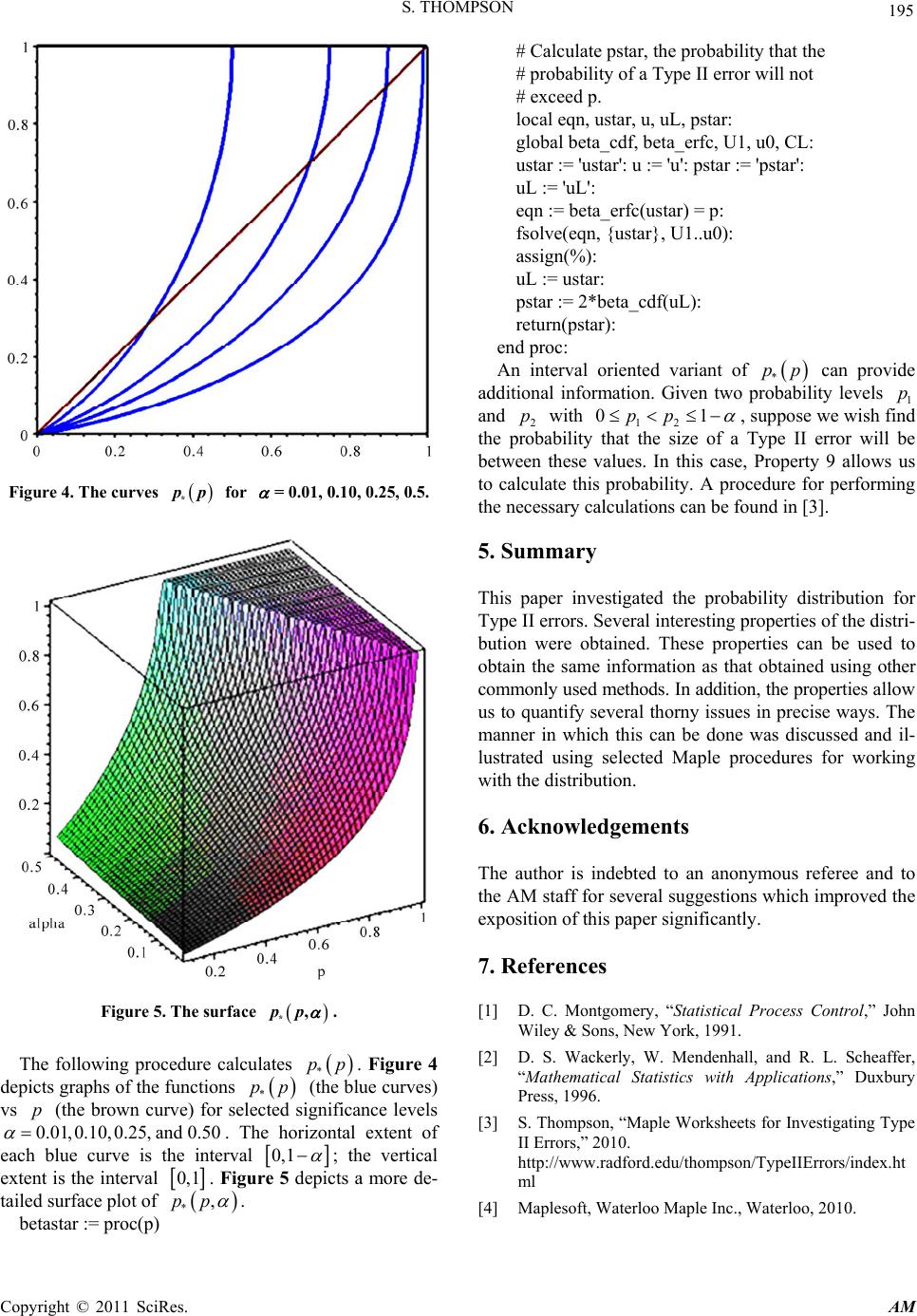

S. THOMPSON
195
Figure 4. The curves

*
pp
for

= 0.01, 0.10, 0.25, 0.5.
Figure 5. The surface


*,

pp .
The following procedure calculates

*
pp. Figure 4
depicts graphs of the functions

*
pp (the blue curves)
vs p (the brown curve) for selected significance levels
0.01,0.10,0.25,and 0.50

. The horizontal extent of
each blue curve is the interval


0, 1

; the vertical
extent is the interval


0,1 . Figure 5 depicts a more de-
tailed surface plot of

*,pp

.
betastar := proc(p)
# Calculate pstar, the probability that the
# probability of a Type II error will not
# exceed p.
local eqn, ustar, u, uL, pstar:
global beta_cdf, beta_e r fc, U1, u0, CL :
ustar := 'ustar': u := 'u': pstar := 'pstar':
uL := 'uL':
eqn := beta_erfc(ustar) = p:
fsolve(eqn, {ustar}, U1..u0):
assign(%):
uL := ustar:
pstar := 2*beta_cdf(uL):
return(pstar):
end proc:
An interval oriented variant of

*
pp can provide
additional information. Given two probability levels 1 p
and 2 p with 12 01pp


, suppose we wish find
the probability that the size of a Type II error will be
between these values. In this case, Property 9 allows us
to calculate this probability. A procedure for performing
the necessary calculations can be found in [3].
5. Summary
This paper investigated the probability distribution for
Type II errors. Several interesting properties of the distri-
bution were obtained. These properties can be used to
obtain the same information as that obtained using other
commonly used methods. In addition, the properties allo w
us to quantify several thorny issues in precise ways. The
manner in which this can be done was discussed and il-
lustrated using selected Maple procedures for working
with the distribution.
6. Acknowledgements
The author is indebted to an anonymous referee and to
the AM staff for several suggestions which improved the
exposition of this paper significantly.
7. References
[1] D. C. Montgomery, “Statistical Process Control,” John
Wiley & Sons, New York, 1991.
[2] D. S. Wackerly, W. Mendenhall, and R. L. Scheaffer,
“Mathematical Statistics with Applications,” Duxbury
Press, 1996.
[3] S. Thompson, “Maple Worksheets for Investigating Type
II Errors,” 2010.
http://www.radford.edu/thompson/TypeIIErrors/index.ht
ml
[4] Maplesoft, Waterloo Maple Inc., Waterloo, 2010.