Paper Menu >>
Journal Menu >>
 Applied Mathematics, 2011, 2, 165-180 doi:10.4236/am.2011.22019 Published Online February 2011 (http://www.SciRP.org/journal/am) Copyright © 2011 SciRes. AM Reservoir Multiscale Data Assimilation Using the Ensemble Kalman Filter Santha R. Akella Department of Earth and Planetary Sciences, Johns Hopkins University, Baltimore, USA E-mail: santha.akella@jhu.edu Received June 22, 201 0; revised November 11, 2010; accepted November 15, 2010 Abstract In this paper we propose a way to integrate data at different spatial scales using the ensemble Kalman filter (EnKF), such that the finest scale data is sequentially estimated, subject to the available data at the coarse scale (s), as an additional constraint. Relationship between various scales has been modeled via upscaling techniques. The proposed coarse-scale EnKF algorithm is recursive and easily implementable. Our numerical results with the coarse-scale data provide improved fine-scale field estimates when compared to the results with regular EnKF (which did not incorporate the coarse-scale data). We also tested our algorithm with var- ious precisions of the coarse-scale data to account for the inexact relationship between the fine and coarse scale data. As expected, the results show that higher precision in the coarse-scale data, yielded improved es- timates. Keywords: Kalman Filter, Reservoir Engineering, Uncertainty Quantification, Multiscale Data 1. Introduction The principal objective of data assimilation methods [1] is to combine the information provided by measured data and a (numerical) forecast model to obtain an improved estimate of the system state (and parameters). Unlike va- riational methods which require availability of complex adjoint models for data assimilation, the ensemble Kal- man filter (EnKF) can be quickly implemented and one can also obtain uncertainty estimates via error variance- covariance propagation; see [2] and references therein for further details. The EnKF is a sequential Monte Carlo method based on Bayes theorem. The method is increa- singly being used for estimating unknown model state and parameters in various geological and hydrological models [3]. One of the major problems in subsurface characteriza- tion is the huge uncertainty in the knowledge of hydro- carbon reservoir permeability and porosity. Since the flow of hydrocarbons such as oil and gas through the subsurface formation critically depends on the geological rock properties, it is important to accurately know these properties. This article focuses on methods to obtain more accurate quantification of the reservoir rock prop- erties using measured data. Broadly speaking, the meas- ured data used for description of reservoir porosity and permeability characterization consist of static and dyna- mic data. Static data such as well logs, core samples can resolve heterogeneity at a scale of a few inches or feet with high reliability. However, dynamic data such as fra- ctional flow (defined as the ratio of the injection fluid to the total fluid produ ced at the production wells; or water cut), pressure transient and tracer test data typically scan the length scales comparable to the inter-well distances. Additional dynamic data such as time-lapse seismic im- ages [4] can provide improved spatial sampling, but at a lower precision. A majority of p reviou s studies on uncer- tainty quantification in reservoir performance forecasting using EnKF have mostly dealt with integration of dy- namic data (for e.g., [5-7]). However it is widely recog- nized that integration of additional multiscale data could further reduce the uncertainty (see [8,9] and references therein). With that perspective, integration of data at coarse-and fine-scales, is an important objective and is addressed in this paper. We use the EnKF to estimate fine-scale fields for subsurface characterization. Also, our method could be generalized to other sequential data assimilation methods such as particle filtering (where, rather than updating the ensemble members model state, we update the probability assigned to each ensemble member based on model data misfit). The main reason why we used EnKF in this paper is because it requires  S. R. AKELLA Copyright © 2011 SciRes. AM 166 fewer ensemble members than the particle filters, see [3] and references therein for further details. In this paper, apart from the water cut data, we consi- der coarse-scale measured data as well. The coarse-scale data is assumed to be permeability at some specified lev- el of precision. The unknown variables: permeability, at the fine-scale, are estimated using a modification to the EnKF algorithm, linking the data at different scales via upscaling. It is important to resolve fine-scale heteroge- neity for various purposes such as, enhanced oil recove- ry, environmental remediation, etc. The main idea behind upscaling is to obtain an effective coarse-scale permea- bility which yields the same average response as that of the underlying fine-scale field, locally. Single phase flow upscaling procedures for two phase flow problem have been discussed by many authors; see e.g., [10,11] and also Section 3.1. We will refer to our proposed v ariant of EnKF as coarse-scale EnKF. Assimilation using dynam- ic data, such as fractional flow data only, is therefore referred to as regular EnKF. The coarse-scale permeabil- ity data could be obtained either from geo logic consider- ation or coarse-scale inversion of dynamic, fractional flow data on a coarse grid as considered in [8,12]. This coarse-scale, static data can be viewed as a constraint, which is to be satisfied up to the prescribed variance for obtaining the fine-scale estimates in every data assimila- tion cycle. Upscaling methods relate the solution at the finescale to the coarse-scale, therefore in the Kalman filter context, it amounts to modeling a nonlinear obser- vation operator. In our coarse-scale EnKF approach, we use the measured data in batches, such that the estimate with one data becomes a prior while assimilating the other observation (see Section 3 for further details). Though in this paper we used coarse-scale data at only one scale, our approach can be easily generalized to as- similate data at multiple scales by appropriately model- ing the linkage between different scales. Also, our ups- caling method is independent of the underlying fine- scale field. For the purpose of self-conten dness an d notationa l cla- rity, we briefly review the governing equations, sequen- tial data assimilation using the ensemble Kalman filter in Section 2, which is followed by a description of the coar- se-scale EnKF algorithm (Section 3). For our numerical results (Section 4), we consider a five-spot pattern, with the injection well placed in the middle of a rectangular domain and four production wells located at the vertices of the rectangle. A reference case is used to provide true data, which is randomly perturbed to obtain synthetic measurements. A comparison of the regular EnKF with the coarse-scale EnKF (Sections 4.1 and 4.2 respectively) shows that using coarse-scale permeability data (via coarse-scale EnKF) significantly improves the fine-scale estimates as well as future fractional flow prediction. 2. Background 2.1. Fine-Scale Model In this paper, we consider two-phase flow in a subsurface formation under the assumption that the displacement is dominated by viscous effects. For simplicity, we neglect the effects of gravity, compressibility, and capillary p res- sure, although our proposed approach is independent of the choice of physical mechanisms. Also, porosity will be considered to be constant. The two phases will be re- ferred to as water and oil (or a non-aqueous phase liquid), designated by subscripts w and o, respectively. We write Darcy’s law for each phase as follows: =; =, rj jf f j kS νκprS κpr h (1) =,= , == ; rwrorw w wo rwwroo wo f kS kSkS SfS kS kS S νν νSκpr νS t (2) The above descriptions are referred to as the fine-scale model of the two-phase flow problem. Here f κ is the (fine-scale) permeability of the medium, S is the total mobility, j denotes phase viscosity, pr is the pressure, h is the source term, and S denote poros- ity and water saturation (volume fraction), respectively. 2.2. Sequential Estimation using EnKF Using dynamic measured data such as water cut, we can sequentially estimate the unknown parameters (permea- bility, porosity, etc.) and state v ariables such as pressure, water saturation (two-phase flow) and production data at well locations using the EnKF as discussed in [5,7,13]. Following these previous works, in th is paper we assume that the only dynamic data available is water cut data, and that porosity is known. The combined state-parameter to be estimated are given by =,,,. T fc ln κ Ψpr S W Where ln is natural logarithm of permeability field and c W denotes water cut; in order to distinguish ob- served water cut from model predicted water cut, now onwards we will denote the observed water cut data o c W, by y . The EnKF introduced in [14] is a sequential Monte Carlo method where an ensemble of model states evolve in state-space with mean as the best estimate and spread of the ensemble as the error covariance, as summarized in the following steps. Each of the ensemble members is  S. R. AKELLA Copyright © 2011 SciRes. AM 167 forecasted independently (in this work, we neglected mo- deling errors), 1=, ii nn F ΨΨ (3) where F is the forecast operator (Equations (1), (2)), superscript i denotes the th i ensemble member; now onwards we will drop the time subscript. The en- semble mean and covariance are defi ned as, =1 1 =, Nei i e N ΨΨ (4) 1'', 1 T f e N PAA (5) where 12 '=,,,, Ne Abb b =, ii bΨΨ and e N is the number of ensemble members. The observa- tion vector for each ensemble member is given by, =, ii t Hν yΨ (6) where t HΨ is the observed data from the truth and i ν represents observational errors, which are i.i.d. samples [15] from a normal distribution with zero mean and variance, .R We note that if only the water cut data is being measured, the mapping from model-to-observa- ti o n al space, H is trivially equal to ,000I since =,,,. T c ln κ Ψpr S W The forecasted ensemble (Equation (3)) is updated by assimilating the observed data, , iii i ΨΨKy HΨ (7) where K is the Kalman gain, given by 1 =. fT fT KPHHPH R Computationally efficient implementation of the EnKF is discussed for e.g., in [2,16]. We use the above set of corrected ensemble states, 0 e N i i Ψ in the simulation model (Equation (3)) to predict until the next set of ob- servational data is available. 3. Coarse-Scale Constrained EnKF The EnKF presented so far, used only the dynamic, pro- duction data (wat er cut) , y with error =t ν yHΨ, ,ν0R to update the ensemble (Equation (7)). In addition to , y if we are also given static data (as men- tioned in the Introduction), which is another set of inde- pendently measured data, .z Assuming that the corres- ponding measurement error is given by =, t ω zUΨ ,;ω0Q :.UΨz Its like- lihood is given by 1 1 exp . 2 T z p zΨzUΨQzUΨ (8) If this static data z, corresponds to coarse-scale per- meability data [12,8], then =.U000Where :, f c κκ is a nonlinear mapping that maps the fine-scale permea- bility field ( f κ) to coarse-scale field (c κ) via an upscal- ing procedure (e.g., [17,18]), details are provided in Sec- tion 3.1. Note that by definition, the errors in water-cut data, y and coarse-scale permeability, c κ data don’t influence each other, since they are entirely differently measured quantities. Now, our goal is to obtain an estimate which is based on both of the above dynamic and static data. The like- lihood of y is given by 1 1 exp . 2 T y p yΨyHΨRyHΨ The probability distribution function (pdf) of the pre- dicted ensemble, 1 1 exp , 2 Tf f p ΨΨΨPΨΨ where Ψ and f P are the predicted ensemble mean and covariance respectively (Equations (4) and (5)). Then, using Bayes theorem, we obtain | ,, |, =, , =, , =. p p pp pp pp p ppp Ψy Ψzy Ψzy zy zyΨΨzyΨΨ zy zΨyΨΨ The last term in above equation implies that the two independent data, y and z can be sequentially assimilated in the following two steps. We first assimilate observa- tion y to obtain an intermediate ensemble, 0 e N i i Ψ as discussed in Section 2. 2. exp , fy ppyΨΨ (9) This intermediate ensemble and likelihood in Equation (8), can then be combined to obtain the final estimate 0 e N i i Ψ. ,exp , fyz ppΨΨzy (10) Therefore, in a least-squared sense, the final estimate maximizes the posterior pdf , p zyΨ which corres- 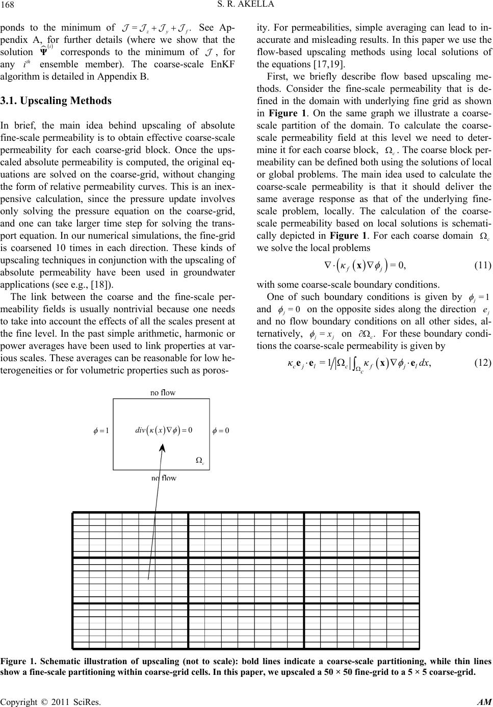 S. R. AKELLA Copyright © 2011 SciRes. AM 168 ponds to the minimum of =. z yf See Ap- pendix A, for further details (where we show that the solution i Ψ corresponds to the minimum of , for any th i ensemble member). The coarse-scale EnKF algorithm is detailed in Appendix B. 3.1. Upscaling Methods In brief, the main idea behind upscaling of absolute fine-scale permeability is to obtain effective coarse-scale permeability for each coarse-grid block. Once the ups- caled absolute permeability is computed, the original eq- uations are solved on the coarse-grid, without changing the form of relative permeability curves. This is an inex- pensive calculation, since the pressure update involves only solving the pressure equation on the coarse-grid, and one can take larger time step for solving the trans- port equation. In our numerical simulations, the fine-grid is coarsened 10 times in each direction. These kinds of upscaling techniques in conjunction with the upscaling of absolute permeability have been used in groundwater applications (see e.g., [18]). The link between the coarse and the fine-scale per- meability fields is usually nontrivial because one needs to take into account the effects of all the scales present at the fine level. In the past simple arithmetic, harmonic or power averages have been used to link properties at var- ious scales. These averages can be reasonable for low he- terogeneities or for volumetric properties such as poros- ity. For permeabilities, simple averaging can lead to in- accurate and misleading results. In this paper we use the flow-based upscaling methods using local solutions of the equations [17,19 ]. First, we briefly describe flow based upscaling me- thods. Consider the fine-scale permeability that is de- fined in the domain with underlying fine grid as shown in Figure 1. On the same graph we illustrate a coarse- scale partition of the domain. To calculate the coarse- scale permeability field at this level we need to deter- mine it for each coarse block, c . The coarse block per- meability can be d efined both using the so lutions of local or global problems. The main idea used to calculate the coarse-scale permeability is that it should deliver the same average response as that of the underlying fine- scale problem, locally. The calculation of the coarse- scale permeability based on local solutions is schemati- cally depicted in Figure 1. For each coarse domain c we solve the local problems =0, fj κ x (11) with some coarse-scale boundary conditions. One of such boundary conditions is given by =1 j and =0 j on the opposite sides along the direction j e and no flow boundary conditions on all other sides, al- ternatively, = j j x on . c For these boundary condi- tions the coarse-scale permeability is given by =1 , cj lcfj l c κκdx eexe (12) 0 1 0div κx c Figure 1. Schematic illustration of upscaling (not to scale): bold lines indicate a coarse-scale partitioning, while thin lines show a fine-scale partitioning within coarse-grid cells. In this paper, we upscaled a 50 × 50 fine-grid to a 5 × 5 coarse-grid.  S. R. AKELLA Copyright © 2011 SciRes. AM 169 where j is the solution of Equation (11) with prescri- bed boundary conditions. Various boundary condition can have some influence on the accuracy of the calculations, including periodic, Dirichlet, etc. These issues have been discussed for e.g., in [19]. In particular, for determining the coarse-scale permeability field one can choose local domains that are larger than target coarse block, c , for Equation (11). Further Equation (12) is used in the do- main c , where j are computed in the larger do- mains with correct scaling (see [19]). This way one re- duces the effects of the artificial boundary conditions imposed on c (for details see [19]). The use of the local solutions Equation (11) for deter- mining the permeability field at different scales gives non-explicit relation for conditional distribution. We denote by the local operator that maps the local fine-scale permeability field f κ into c κ, defined as above. For our computations we assume =, cf κκ (13) where are some random fluctuations that represent inaccuracies in the coarse-scale permeability. In reality, since we do not have the fine-scale field, f κ available, it is difficult to characterize the exact (nature of the) er- ror in upscaling. However, one of the sources of these fluctuations are the errors associated with solving inv erse problems on the coarse grid. The other source of the in- accuracies of measured coarse-scale permeability is due to the fact that the inversion on the coarse grid does not take into account the adequate form of the coarse-scale models. Here we assumed these errors to be normally distributed (further details follow in Section 4.2). 4. Numerical Results For our numerical tests with the coarse-scale EnKF algo- rithm, we use a 50 50 fine grid (dimensionless do- main size 50 50). We consider the coarse-scale per- meability, which could be obtained by coarse-scale in- version of fractional flow data on a coarse grid [12,20]. This coarse-scale field could be thought as static data, which is to be honored as constraint (up to the data va- riance) in Equation (8), hence we need to always assimi- late it in our coarse-scale EnKF algorithm. An initial ensemble with different permeability reali- zations was generated using the sequential Gaussian si- mulation (SGSIM)1 [22]. We specified a Gaussian vario- gram model with a correlation length of 20 gridblocks in the x-direction and 5 gridblocks in the y-direction; one of the realizations is used as the reference field (depicted in Figure 2). The fractional flow will be calculated based on the fine-scale model in Section 2.1. Porosity ( ) is assumed to be equal to 0.15 for all grid blocks. For sim- plicity, relative permeabilities, rj k are assumed to be linear functions of water saturation (S): =, rw kS S =1 . ro kS S One injection well at the center of the field (injection rate: 71.4 m3/day) and four producing wells at the four corners (all with equal rate of 17.85 m3/day) were considered. The model equations are sol- ved with no flow boundary conditions, zero initial water saturation, and discretizing the transport equation using first order upwind finite volume method. In Figure 3, we provide the predicted fractional flow for 256 initial en- semble members along with the true fractional flow (ob- tained from true permeability field). To compare our proposed coarse-scale constrained EnKF results with the regular EnKF we will use the fol- lowing mean 2 L-norm error. Since we know the true (fine and coarse-scale) field for our synthetic problem, i.e., the true permeability field, denoting it by , true κ the error for any ensemble member is =,=1,2,,. ii true e κκiNe Consider the 2 L norm of the error for each member, 2 2=, ii j j ee using which we define the mean 2 L error as 2 =1 1 =, Ne i i e N ee (14) so that e gives us an indication of the distance of entire ensemble from the true solution . true κ Since after every Figure 2. Natural logarithm of 50 × 50 true permeability field. 1For reservoir simulation applications, the SGSIM has been used [21, 13] for generating initial ensemble members. This approach yields independent and identically distributed multivariate normal rando m fields (conditioned to well log data)  S. R. AKELLA Copyright © 2011 SciRes. AM 170 Figure 3. Fractional flow prediction with 256 initial ensemble members (no data assimilation); ensemble members (green dots), ensemble mean (blue crosses) compared with true water cut data (red open circles). observation, we have updated ensemble members, there- fore we can monitor the variation of e over the time of assimilation; the success of assimilation can therefore be related to the decrease in e. 4.1. EnKF with Fractional Flow Data Only We start with a presentation of results with regular EnKF, assimilating only water cut data. Next we will discuss results with the coarse-scale EnKF. The water cut data from the reference field is assumed to be available every 200 days, with mean zero and standard deviation of 0.01 (therefore 1/24 =0.01 ,RI where 4 I is unit matrix of size 44, since there are four producing wells). The observed data is assumed to be available up to 2400 days, hence we will perform as- similation between 200 and 2400 days. A prediction beyond interval of data assimilation, up to 4000 days is also provided. We selected an ensemble of size 256 for presenting our data assimilation results. We assimilated the above described measured data, and using the assimilated permeability field, in Figure 4 we plot the assimilated water cut data along with the true data. Comparing with the initial forecast in Figure 3, we observe that the assimilated ensemble better envelopes the true data. We compare the initial permeability field before assimilation (Figure 5(a)-(d)) for a few ensemble members with the true field in Figure 2 and with those obtained after assimilation in Figure 6(a)-(d); note that the central, South East-North West channel is prominent but the features at the South West and North East corners are not well captured. Therefore assimilation of only water cut data helps in identifying only some of the im- portant features. 4.2. Coarse-Scale Constrained EnKF with Fractional Flow and Coarse-Scale Permeability Data In addition to water cut production data, the coarse-scale  S. R. AKELLA Copyright © 2011 SciRes. AM 171 Figure 4. Water cut prediction using assimilated (regular EnKF for 2400 days) ensemble members, note the improved fit of ensemble when compared to that in Figure 3. permeability data, as described in Section 3.1 has been used as additional measured data. Flow-based upscaling of reference permeability field is used as a proxy for in- verted coarse field. Following our previous notation, this coarse-scale permeability data will be denoted by z (Equation (8)). The mapping between state variables (at fine-scale) and observations (at coarse-scale) is given by =,U000 , denotes flow-based upscaling. Exactly as in the previous section, we prescribed the same frequency (of availability) and precision, R for the fractional flow data. Since we use coarse-scale permea- bility as additional data, it is to be assimilated whenever we assimilate water cut data. A 5 × 5 coarse-scale data with mean zero and variance, 25 =QqI (we will present results with =4,2,1,0.5q and 0.1,) so that we can con- sider the impact of coarse-scale data precision. In Figure 7 we plot the variation of mean 2 L error, e (Equation (14)) with observation time, at the coarse-scale for dif- ferent values of .q Figures 8(a) and (b) depict the cor- relation between coarse-scale ensemble mean and true fields for q = 4 and 0.1, respectively. As the precision of coarse-scale data is increased, i.e., for smaller variance, we observe a larger decrease in coarse-scale mean 2 L error and higher correlation with true coarse-scale field (correlation coefficient for =4,2,1,0.1q respectively are 0.976, 0.992, 0.995, 0.999), b ecause smaller variance Q implies more stricter coarse-scale data constraint in Equation (8). Figure 9(a)-(d) depict the fractional flow using the final permeability field after assimilation, for different coarse-scale data precisions. Figures 7 and 8(a)-(b) show that the coarse-scale data is being more accurately assimilated as it is made more precise. Also, notice the improv ed fit of ense mble predictio n to the tru e data, for more precise coarse-scale data; also when com- pared to the regular EnKF results in Figure 4. Now we discuss the results regarding fine-scale field. In Figure 10 we plot the fine-scale mean 2 L error for different values of ;q the coarse-scale EnKF yields much lesser error than regular EnKF which assimilated only fractional flow data. The correlation coefficient  S. R. AKELLA Copyright © 2011 SciRes. AM 172 (a) (b) (c) (d) Figure 5. Log permeabilities of a few i-th. initial ensemble members (before data assimilation); left-right, (a) i = 50, (b) 100, (c) 150, (d) 200. (a) (b) (c) (d) Figure 6. Same as above, but after assimilating water cut data with regular EnKF. 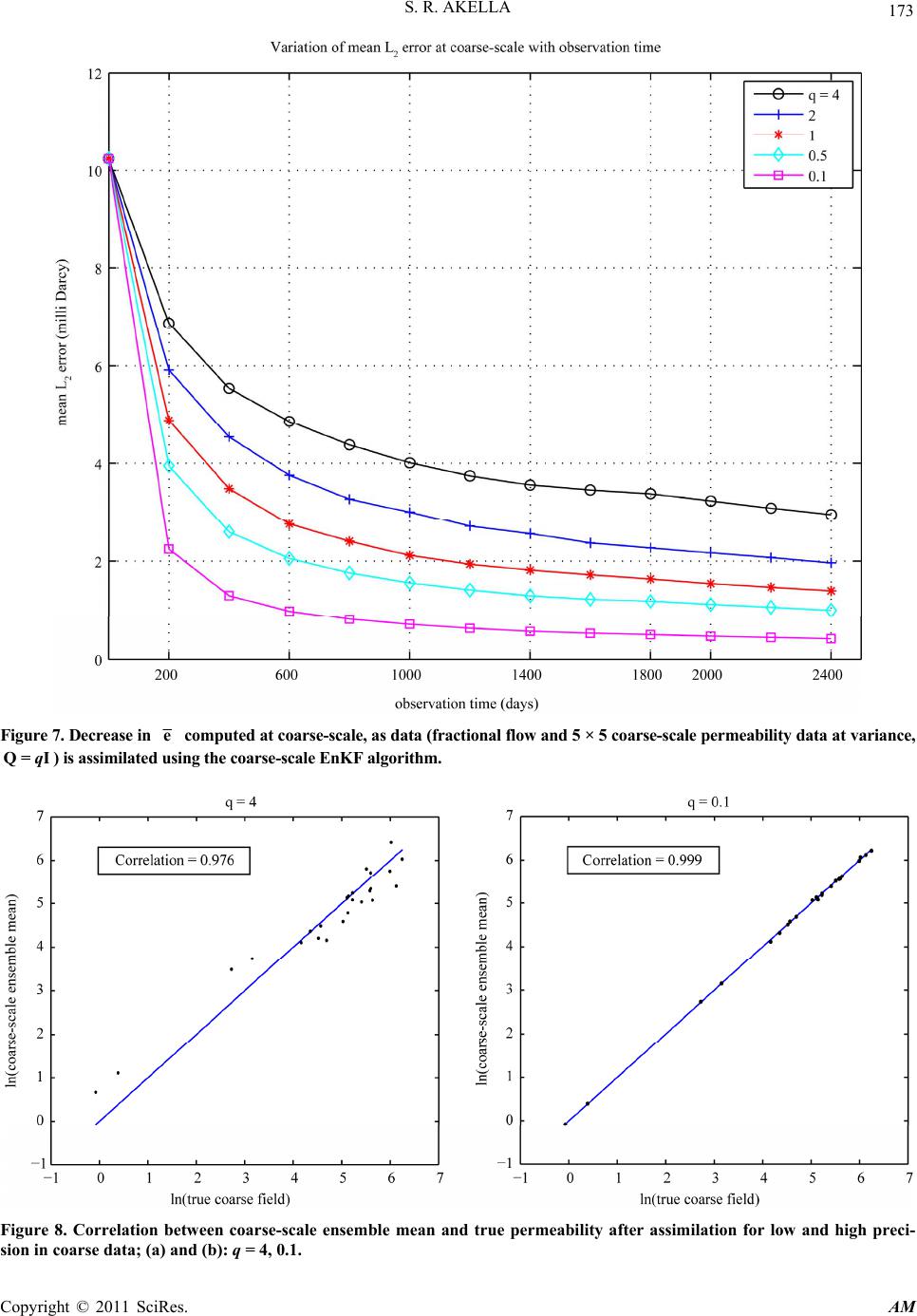 S. R. AKELLA Copyright © 2011 SciRes. AM 173 Figure 7. Decrease in e computed at coarse-scale, as data (fractional flow and 5 × 5 coarse-scale permeability data at variance, Q= I q ) is assimilated using the coarse-scale EnKF algorithm. Figure 8. Correlation between coarse-scale ensemble mean and true permeability after assimilation for low and high preci- sion in coarse data; (a) and (b): q = 4, 0.1. 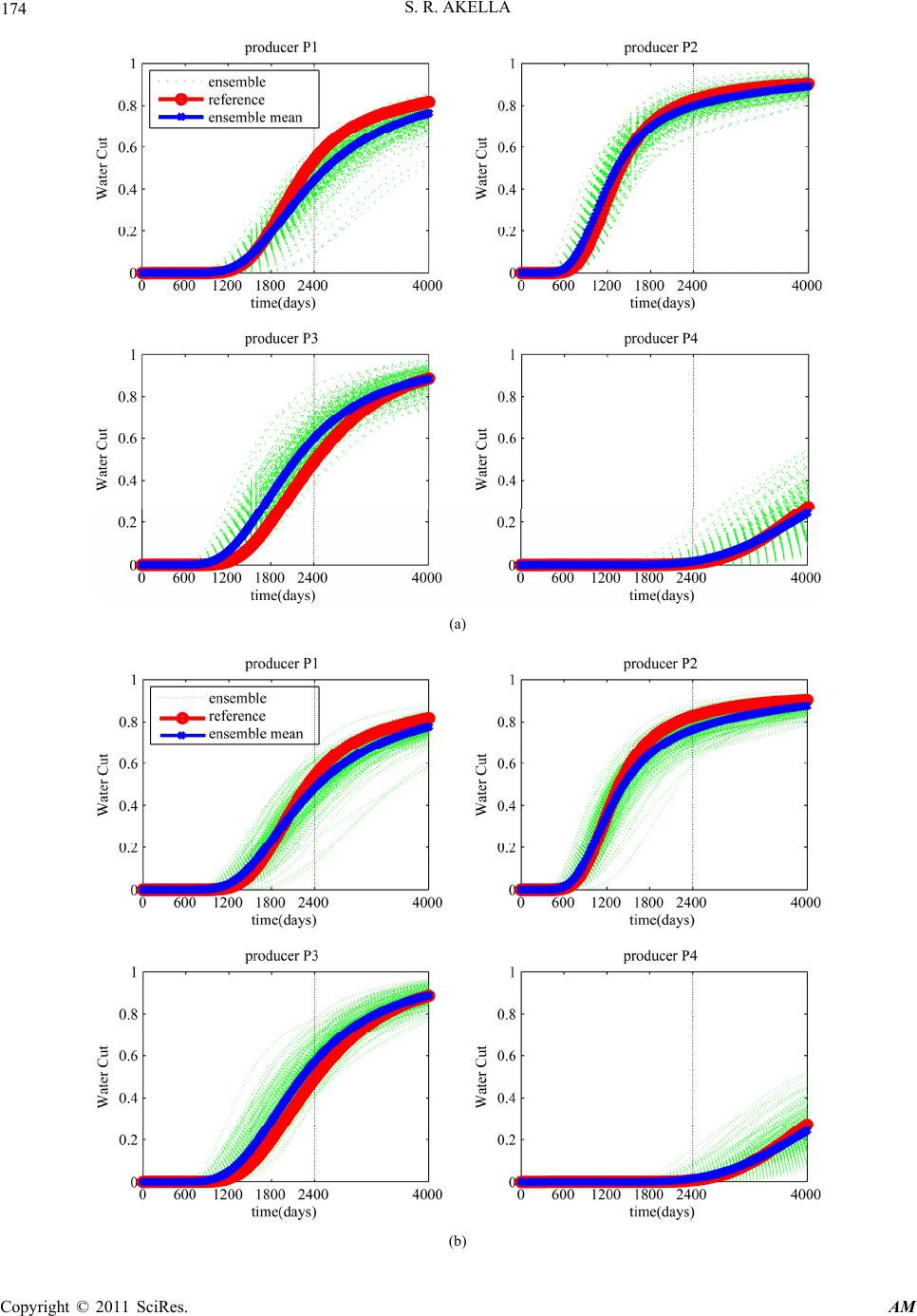 S. R. AKELLA Copyright © 2011 SciRes. AM 174 (a) (b) 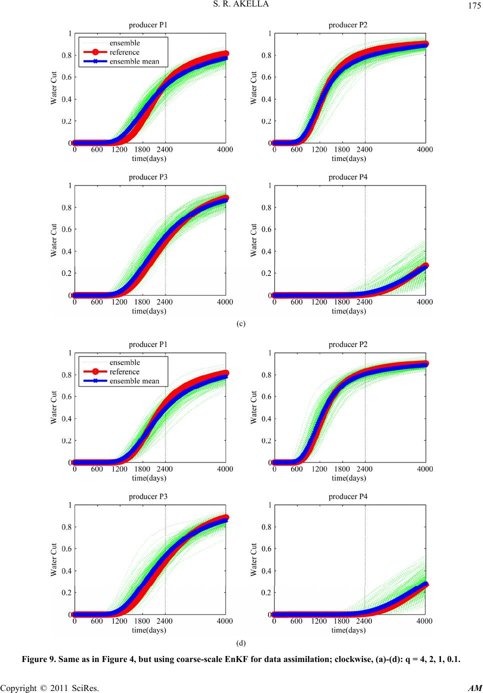 S. R. AKELLA Copyright © 2011 SciRes. AM 175 (c) (d) Figure 9. Same as in Figure 4, but using coarse-scale EnKF for data assimilation; clockwise, (a)-(d): q = 4, 2, 1, 0.1. 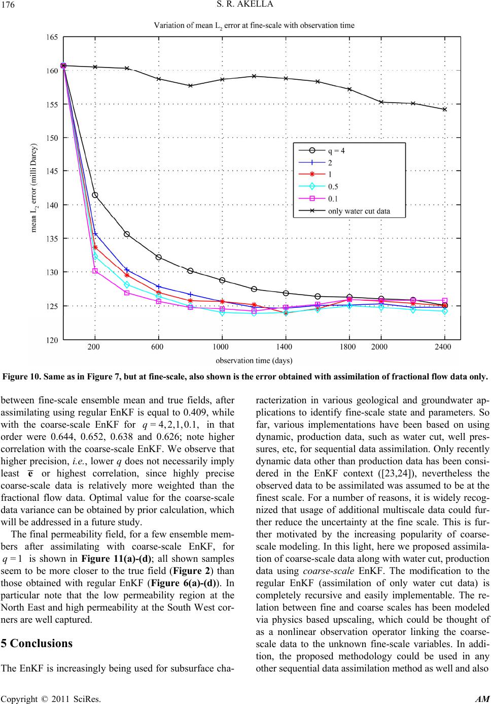 S. R. AKELLA Copyright © 2011 SciRes. AM 176 Figure 10. Same as in Figure 7, but at fine-scale, also shown is the error obtained with assimilation of fractional flow data only. between fine-scale ensemble mean and true fields, after assimilating using regular EnKF is equal to 0.409, while with the coarse-scale EnKF for =4,2,1,0.1,q in that order were 0.644, 0.652, 0.638 and 0.626; note higher correlation with the coarse-scale EnKF. We observe that higher precision, i.e. , lower q does not necessarily imply least e or highest correlation, since highly precise coarse-scale data is relatively more weighted than the fractional flow data. Optimal value for the coarse-scale data variance can be obtain ed by prio r calculation, which will be addressed in a future study. The final permeability field, for a few en semble mem- bers after assimilating with coarse-scale EnKF, for =1q is shown in Figure 11(a)-(d); all shown samples seem to be more closer to the true field (Figure 2) than those obtained with regular EnKF (Figure 6(a)-(d)). In particular note that the low permeability region at the North East and high permeability at the South West cor- ners are well capt ured. 5 Conclusions The EnKF is increasingly being used for subsurface cha- racterization in various geological and groundwater ap- plications to identify fine-scale state and parameters. So far, various implementations have been based on using dynamic, production data, such as water cut, well pres- sures, etc, for sequential data assimilation. Only recently dynamic data other than production data has been consi- dered in the EnKF context ([23,24]), nevertheless the observed data to be assimilated was assumed to be at the finest scale. For a number of reasons, it is widely recog- nized that usage of additional multiscale data could fur- ther reduce the uncertainty at the fine scale. This is fur- ther motivated by the increasing popularity of coarse- scale modeling. In this light, here we proposed assimila- tion of coarse-scale data along with water cut, production data using coarse-scale EnKF. The modification to the regular EnKF (assimilation of only water cut data) is completely recursive and easily implementable. The re- lation between fine and coarse scales has been modeled via physics based upscaling, which could be thought of as a nonlinear observation operator linking the coarse- scale data to the unknown fine-scale variables. In addi- tion, the proposed methodology could be used in any other sequential dat a assimilation m ethod as wel l and al so  S. R. AKELLA Copyright © 2011 SciRes. AM 177 (a) (b) (c) (d) Figure 11. Same as in Figure 6, but assimilated using coarse-scale EnKF with q=1 for the variance of coarse-scale permeabil- ity data. also with any other upscali n g method. The coarse-scale EnKF was tested and compared with the regular EnKF for a 2D synthetic 50 50 heteroge- nuous true field. We considered coarse-scale permeabil- ity data as additional data on a 55 coarse grid. This coarse-scale data was always assimilated along with wa- ter cut data. The data variance was varied from low to high, to study its impact on assimilated results. In all cases, we observed that the assimilated, ensemble mean coarse-scale field for all variances was highly correlated to the true coarse-scale field. In addition, lower variance in the coarse-scale data yielded higher correlation. The water cut data was better h onored, both for higher preci- sion of coarse data, and when compared with regular EnKF. As for the fine-scale permeability field, the coarse-scale EnKF yielded lesser error in an averaged 2 L norm, error taken w.r.t. the reference field. In addi- tion, a few individual samples were picked to compare the assimilated fields with different EnKF procedures; experiment with coarse-scale permeability data provided final samples which captured most closely the features in the reference fine-scale field. Though in our current paper we used only one coarse- scale, the proposed method can be easily implemented to integrate as many scales as required by the available data and is independent of the underlying fine-scale field. Based on our results we conclude that there could be a singinificant improvement in subsurface characterization if accurate and additional data at coarse-scales is availa- ble. In future we plan to study the nature of errors in- volved in coarse-scale data and upscaling and in-turn their influence on the proposed coarse-scale EnKF. 6. References [1] J. M. Lewis, S. Lakshmivarahan and S. Dhall, “Dynamic Data Assimilation: A Least Squares Approach (Encyclo- pedia of Mathematics and its Applications),” Cambridge University Press, Cambridge, 2006. doi:10.1017/CBO 9780511526480 [2] G. Evensen, “Data Assimilation: The Ensemble Kalman Filter,” Springer, Berlin, 2006. [3] Y. Liu and H. V. Gupta, “Uncertainty in Hydrologic Modeling: Toward and Integrated Data Assimilation Framework,” Water Resources Research, Vol. 43, 2007, W07401. doi:10.1029/2006WR005756 [4] D. E. Lumley, “Time-Lapse Seismic Reservoir Monitor- ing,” Geophysics, Vol. 66, No. 1, 2001, pp. 50-53. doi:10.1190/1.1444921 [5] G. Nævdal, L. Johnson, S. Aanonsen and E. Vefring, “Reservoir Monitoring and Continuous Model Updating  S. R. AKELLA Copyright © 2011 SciRes. AM 178 Using Ensemble Kalman Filter,” SPE Journal, Vol. 10, No. 1, 2005, pp. 66-74. [6] X.-H Wen and W. H. Chen, “Real-Time Reservoir Model Updating Using Ensemble Kalman Filter,” Proceedings of SPE Reservoir Simulation Symposium 2005, SPE 92991, 31 January-2 February 2005, Texas. [7] Y. Q. Gu and D. S. Oliver, “The Ensemble Ka lman Filter for Continuous Updating of Reservoir Simulation Mod- els,” Journal of Energy Resources Technology-Transac- tions of the ASME, Vol. 128, 2006, pp. 79-87. doi:10.1115/1.2134735 [8] S. H. Lee, A. Malallah, A. Datta-Gupta and D. Higdon, “Multiscale Data Integration Using Markov Random Fields,” SPE Reservoir Evaluation Engineering, Vol. 5, 2002, pp. 68-78. doi:10.2118/76905-PA [9] Y. Efendiev, A. Datta-Gupta, V. Ginting, X. Ma and B. Mallick, “An Efficient Two-Stage Markov Chain Monte Carlo Method for Dynamic Data Integration,” Water Re- sources Research, Vol. 41, 2005, doi:10.1029/2004WR003764 [10] M. Christie, “Upscaling for Reservoir Simulation,” Jour- nal of Petroleum Technology, Vol. 48, No. 11, 1996, pp. 1004-1010. doi:10.2118/37324-MS [11] J. W. Barker and S. Thibeau, “A Critical Review of the Use of Pseudo-Relative Permeabilities for Upscaling,” SPE Reservoir Engineering, Vol. 12, 1997, pp.138-143. doi:10.2118/35491-PA [12] Y. Efendiev, A. Datta-Gupta, I. Osako and B. Mallick, “Multiscale Data Integration Using Coarse-Scale Mod- els,” Advances in Water Resources, Vol. 28, No. 3, 2005, pp. 303-314. doi:10.1016/j.advwatres.2004.10.013 [13] D. Devegowda, E. Arroyo-Negrete and A. Datta-Gupta, “Efficient and Robust Reservoir Model Updating Using Ensemble Kalman Filter with Sensitivity-Based Cova- riance Localization,” Proceedings of SPE Reservoir Si- mulation Symposium, Houston, February 2007. doi:10.2118/106144-MS [14] G. Evensen, “Sequential Data Assimilation with a Nonli- near Quasi-Geostrophic Model Using Monte Carlo Me- thods to Forecast Error Statistics,” Journal of Geophysi- cal Research, Vol. 99, 1994, pp. 143-162. doi:10.1029/94JC00572 [15] G. Burgers, P. J. van Leeuwen and G. Evensen, “Analysis Scheme in the Ensemble Kalman Filter,” Monthly Weather Review, Vol. 126, No. 6, 1998, pp. 1719-1724. doi:10.1175/1520-0493(1998)126<1719:ASITEK>2.0.C O;2 [16] Y. Chen and D. Zhang, “Data Assimilation for Transient Flow in Geologic Formations Via Ensemble Kalman Fil- ter,” Advances in Water Resources, Vol. 29, 2006, pp. 1107-1122. doi:10.1016/j.advwatres.2005.09.007 [17] L. J. Durlofsky, “Numerical Calculation of Equivalent Grid Block Permeability Tensors for Heterogeneous Porous Media,” Water Resources Research, Vol. 27, No. 5, 1991, pp. 699-708. doi:10.1029/91WR00107 [18] L. J. Durlofsky, “Coarse Scale Models of Two Phase Flow in Heterogeneous Reservoirs: Volume Averaged Equations and Their Relationship to the Existing Upscal- ing Techniques,” Computational Geosciences, Vol. 2, 1998, pp. 73-92. doi:10.1023/A:1011593901771 [19] X. H. Wu, Y. R. Efendiev and T. Y. Hou, “Analysis of Upscaling Absolute Permeability,” Discrete and Conti- nuous Dynamical Systems, Series B, Vol. 2, 2002, pp. 185-204. doi:10.3934/dcdsb.2002.2.185 [20] S. Yoon, A. H. Malallah, A. Datta-Gupta, D. W. Vasco and R. A. Behrens, “A Multiscale Approach to Produc- tion-Data Integration Using Streamline Models,” SPE Journal, Vol. 6, No. 2, 2001, pp. 182-192. [21] Y. Gu and D. S. Oliver, “History Matching of the PUNQ-S3 Reservoir Model Using the Ensemble Kalman Filter,” SPE Journal, Vol. 10, No. 2, 2005, pp. 217-224. doi:10.2118/89942-PA [22] C. V. Deutsch, “Journel A. GSLIB: Geostatistical Soft- ware Library and User’s Guide,” Oxford Univiversity Press, Oxford, 1992. [23] Y. Dong , Y. Gu and D. S. Oliver, “Sequential Assimila- tion of 4D Seismic Data for Reservoir Description Using the Ensemble Kalman Filter,” Journal of Petroleum Science and Engineering, Vol. 53, 2006, pp. 83-99. doi:10.1016/j.petrol.2006.03.028 [24] J.-A. Skjervheim, G. Evensen, S. Aanonsen, B. Ruud and T. Johansen, “Incorporating 4D Seismic Data in Reser- voir Simulation Models Using Ensemble Kalman Filter,” SPE Journal, Vol. 12, No. 3, 2007, pp. 282-292. doi:10.2118/95789-PA  S. R. AKELLA Copyright © 2011 SciRes. AM 179 Appendix A: Two Step Coarse-Scale Constrained Kalman Filter Estimate From Section 3, 1 1 =, 2 Tf f ΨΨ PΨΨ and 1 1 =. 2 T y yHΨRyHΨ For notational simplicity we will denote Ψ μ as μ and denote f P by .B Step 1 (minimize f y ): First we minimize the sum, 1=. f y The gra- dient2 of above quadratic cost functional with respect to (w.r.t.) Ψ is given by 11 1=. T ΨBΨHRy HΨμ Then the minimizer μ , of 1 satisfies (we assume H to be linear) 11 =0. T BHRyH μμμ Rearranging the above equation we get, 111 1 =. TT B HRHBHRy μμ (15) Note that the Hessian of 1 w.r.t. Ψ is given by 11T BHRH and for linear quadratic cost functionals, the Hessian inverse is equal to the error covariance ma- trix. Therefore the error covariance matrix, B for μ is given by 1 11 . T BB HRH (16) Step 2 (minimi ze g z ): We use , μ B in 1 1. 2 T g ΨBΨ μ μ 1 1 =. 2 T zQ zUΨzUΨ Therefore the minimum , μ of g z satisfies 11 11 ˆ. TT B UQUBUQz μμ Using Equations (16) and (15) we can rewrite above as 1 11 1 111 .. (14) ˆ . TT TT rh s ofeqation B BHRHUQU BHRyUQz μ μ It is trivial to show that ˆ μ also satisfies =0. fyz Ψ Therefore the two step method to obtain the final es- timate ˆ μ , gives the same results as a one shot approach of minimizing f yz . Appendix B: The Coarse-Scale EnKF Algorithm Run the simulation model up to a particular observation time for entire ensemble to get predicted samples: =1 , Ne i i Ψ 12 =,,, . Ne AΨΨ Ψ 1) Step 1: Using measured water cut data y with vari- ance ,R get updated ensemble: =1 , Ne i i Ψ Step 1.1 Find ensemble mean (Equation (4)), .Ψ Step 1.2 Subtract deviation from mean 12 '=,,,, Ne Abb b =. ii bΨΨ Step 1.3 Apply H to each column of 'A to get ='.SHA i.e., simply pick the water cut deviations in 'A. Step 1.4 for =1,2, ,, e iN Sample i.i.d. ,. i ν0R =, ii νyy 12 12 =,,, , Ne νν νR 12 =,,, , Ne Ddd d =; ii i c dyW i c W is predicted water cut for each ensemble member. end for Step 1.5 Compute SVD 1/2=. L R SRX X Get ˆ retaining first few singular values which explain most variability in , corresponding left singular vectors: . L X Step 1.6 Update ensem ble: Eqnuation ( 7), 12 ,,, e N AΨΨ Ψ, 2 ˆˆ ˆ. TT LL AAASX XD 2) Step 2: Using coarse-scale data z with variance Q, get updated ensemble: =1 . Ne i i Ψ Step 2.1 Compute coarse-scale ensemble prediction: ,1,2,,. i i e iNuUΨ Step 2.2 Coarse-scale mean: =1 1 '= . Ni e i e Nuμ Step 2.3 Coarse-scale deviations: 12 '=,, ,, Ne Ssss ='. ii su μ Step 2.4 Repeat Step 1.4, using coarse-scale mea- 2We note in passing that B and R are covariance matrices and are posi- tive definite by construction, and hence for our derivation purposes, are formally invertible.  S. R. AKELLA Copyright © 2011 SciRes. AM 180 surement. for =1,2, ,, e iN Sample i.i.d.,. i ω0R =, ii ωzz 12 1/2=,,, , Ne ωω ωQ 12 '=,, ,, Ne Ddd d =. iii dzu end for Step 2.5 Compute SVD 1/2 '=. L R SQ XX Get ˆ and L X as in step 1.5 Step 2.6 Compute fine-scale mean: =1 1 '= . Ni e i e N μΨ Step 2.7 Compute fine-scale deviations: 12 =,,,, Ne Abbb ii bΨ μ . Step 2.8 Update ensem ble: 12 ,,, , Ne AΨΨΨ 2 ˆˆ ˆ TT LL AAA SXXD . Remark 1: Note that steps 2.6 and 2.7 in above algorithm approx- imate the intermediate fine-scale error covariance 1. 1 T f e N PAA Remark 2: Steps 2.1-2 . 3 a cc omplish3 '= . SUA Note that the above algorithm is independent of the choice of upscaling procedure and also, we can use the same algorithm for different kinds of coarse-scale ob- served data (if available). Remark 3: Note tha t the above coar se-scale cons trained EnKF algo - rithm can be readily extended to incorporate data at mul- tiple coarse scales, with appropriate upscaling procedure in .U To elaborate, if we had another independent data at a scale different from ,z we use the estimates ( =1 . Ne i i Ψ) obtained using ,z as intermediate solution, repeat Step 2 to assimilate the data at another scale. 3As noted in [2], this approach of accounting for nonlinear observations operator U, works well, as long as U is weakly nonlinear and a mono- tonic function of model variables Ψ. |

