 Journal of Applied Mathematics and Physics, 2013, 1, 68-72 http://dx.doi.org/10.4236/jamp.2013.14013 Published Online October 2013 (http://www.scirp.org/journal/jamp) Copyright © 2013 SciRes. JAMP An Efficient Pattern Search Method Xiaoli Zhang, Qinghua Zhou, Yue Wang College of Mathematics and Computer Science, Hebei University, Baoding, 071002, Hebei, China Email: z xl.hbu@gmail.com, qinghua.zhou@gmaill.com Received June 2013 ABSTRACT Pattern search algorithms is one of most frequently used methods which were designed to solve the derivative-free op- timization problems. Such methods get growing need with the development of science, engineering, economy and so on. Inspired by the idea of Hooke and Jeeves, we introduced an integer in the algorithm which controls the number of steps of iteration update. W e mean along the descent direction, we allow the algor ithm to go ahead steps at most to explore whether we can get better solution further. The experiment proved the strategy’s efficiency. Keywords: Unconstrained Optimization; Derivative-Free Optimization; Pattern Search Methods; Pos itive Bases 1. Introduction In this paper, we consider the unconstrained minimiza- tion pro bl e m where , is continuously differentiable, but the information about the gradient of is either un- available or unreliable. There are lots of problems where derivatives are unavailable but we also want to do some optimizations. The diversity of applications comes from different complicated backgrounds with economics, en- gineering, mathematics, finance, and so on (see [1-3] for instance). In such cases, derivative-free optimization methods (also named direct search methods) which neither com- pute nor approximate derivatives play an important role. The reader is referred to see [4-6]. In [5], the author in- troduced an ingenious idea for a generalized pattern search method and gave convergence analysis. It in- cludes several known algorithms as its special cases. Fa- miliar with the analysis of th e property of the gen eralized method, the author developed two new classes of pattern search methods [6]. Inspired by the idea of Hooke and Jeeves [7], we im- proved the method of [6] by introducing an integer . We mean, if a step is successful (the value of de- crease), then the same direction maybe also be proved successfully at the current point. So, we allow the algo- rithm to explore the same direction further. On the other hand, if it always goes ahead along one direction until it can not improve the value of any more, it likely neglects additional information which other directions can offer. To balance these two aspects, we introduce an integer be used to control iteration steps which we mean that we allow the algorithm to iterate at most steps along the same direction. Next, we would like to present some basic concepts we need. 2. Pattern Search Methods and Positive Bases We use and to represent the Euclidean norm and inner product, respectively. By abuse of nota- tion, if is a matrix, means that the vector is a column of . It will also be convenient to assume that represents, not only the matrix with columns, but also, depending on the context, the set of vectors . The identity matrix is denoted by and its column by . Finally, we write to represent a vector of ones with appropri- ate size. 2.1. Positive Bases We present a few basic properties of positive bases be- ginning from the theory of positive linear dependence developed by Davis [8]. The positive span of a set of vectors is the convex cone 1 {:,0,1,2,, } r nii i i vR vavir α = ∈ =≥= ∑ The set is said to be positively de- pendent if one of the vectors is in the convex cone posi- tively spanned by the remaining vectors, i.e., if one of the vectors is a positively combination of the others; other- wise the set is positively independent. A positive basis is  X. L. ZHANG ET AL. Copyright © 2013 SciRes. JAMP a positively independent set whose positive span is . Alternatively, a positiv e basis for can be defined as a set of nonzero vectors of whose positive combina- tions span is , but no proper set does. The following theorem in [8] indicates that a positive spanning set con- tains at least vectors in . Theorem 1 If positively spans , then it contains a subset with elements that spans . Furthermore, a positive basis can not contain more than elements ([8]). Positive basis with and elements are referred to as minimal and maximal positive basis respectively. We present now three necessary and sufficient char a c- terizations for a set of vectors that spans or spans positively ([8]). Theorem 2 Let , with for all , span . Then the following are equivalent: i) positively spans for . ii) For every , is in the convex cone positively spanned by the remaining vectors. iii) There exist real scalars with , , such that . iv) For every nonzero vector , there exists an index in for with . The following result provides a simple mechanism for generating different positive bases. The proof can be found in [6]. Theorem 3 Suppose is a positive ba- sis for and is a nonsingular matrix, then is also a positive basis for . From above theorems, we can easily deduce the fol- lowing corollary. Corollary 1 Let be a nonsingular matrix, then is a positive basis for . A trivial consequence of this corollary is that is a positive basis. 2.2. Pattern Sea rch Methods Pattern search methods are characterized by the nature of the generating matrices and the exploratory moves algo- rithms. These features are discussed more fully in [5] and [9]. To define a pattern, we need two components, a basis matrix and a generating matrix. The basis matrix can be any nonsingular matrix × ∈. The generating matrix is a matrix , where . We partition the ge- nerating matrix into components We require that , where is a finite set of integral matrices with full row rank. We will see that must have at least columns. The 0 in the last column of is a single column of zeros. A pattern is then def i n ed by the columns of the matrix . For convenience, we use the parti- tion of the generating matrix to partition as follows: Given , we define a trial step to be any vector of the form , where is a to be any vector of the form , column of . Note that determines the direction of the step, while serves as a step length parameter. At the iteration process, we define a trial point as any point of the form , where is the current iteration point. The following algorithms state the pattern search me- thod for unconstr a i ne d minim i z a tion. 2.3. Algorithm 1 Pattern Search Method Let and 00∆> be give n. For Compute . Determine a step using an unconstrained explora- tory moves algorithm. If , then , otherwise . Update and . 2.4. Algorithm 2 Updating Let , and , . Let . If , then . If , then . 3. Our Algorithm and Numerical Results In [5], the generating matrix has the form for some nonsingular matrix . In light of the above discussion, the nature of as a maximal positive basis is now revealed. In [6], the author reduced the number of objective evaluations in the worst case from to as few as . The choice is to make include col- umns which are just the minimal positive bases. In this paper, we simply select the relative parameters as follows: with , . Then, we have all we need to state our algorithm now.  X. L. ZHANG ET AL. Copyright © 2013 SciRes. JAMP Algorithm 3 Modified Pattern Search Method (1) Start with and . (2) Check the stopping criteria. (3) Let and compute . If then go to step (4), else go to step (5). (4) If , then and compute . If , then , go to step (4); else , , go to step (5). (5) If , then , go to step (3); else set 11 1 ,,1, 1 2 k kkk xxkk i ++ = ∆=∆=+= , go to step (2). In fact, from the above algorithms, we can see that if we think any successful step as an iteration , the n in our algorithm should be (identity matrix) or (A matrix which exchanges the row (or column) and the one of the identity matrix). Whenever a step is found failure, then is set to be again. It is easy to know that our choices and settings satisfied the condi- tions in [5,6]. Then, we would like to state the conver- gence theorem which is also the same as in [5,6]. Theorem 4 Assume that is compact and that is continuously differentiable on a neighborhood of . Then for the sequence of iterates gener- ated by algorithm 3, we have . Proof: The reader is referred to [5,6]. Re mark : is Level set defined as follows: ()( )( ) { } 00 , n Lxxfxfxx R=≤∈ . We tested our algorithm on the 18 examples given by Moré, Garbow and Hillstrom [9]. The 19-th is our testing problem at the beginning which we used for testing the effectiveness of the new algorithm. Its definition is: . We select to equal 0, 1, 2, 3, 5 and 10 respectively. It is easy to know that when , it is just the traditional pattern search method with posi- tive basis. The column “P” denotes the number of the problems, and ”N ” the number of variables. The numerical results are given by “F” which denotes the number of function evaluations. And “f” denotes the final function value we got when = 2. Additionally, the symbols “×” means that the algorithm terminates because the number of function evaluation exceeds 500,000. And for the easy comparing among the results we rearranged the order of the number of problems. The stopping condition we select is , (1) which is different with other relative documents. We select Equation (1) as the stopping criteria just be- cause it is simple and easy for understanding. It is thought that if very small step can not lead to decrease in function value, then the current iteration point maybe located in a neighborhood of a local minimum. The algo- rithm is also terminated if the nu mber of function eva lua- tions exceeds 500,000. And we test it from three kinds of initial points, say, , 10 and 100 . The values of them are suggested in [10]. We will see that our algo- rithm is robust and performs the best when m = 2. The results are represented in the following tables in the Ap- pendix. 4. Acknowledgements We are very grateful to the referees for their valuable comme nt s an d suggestio ns. REFERENCES [1] A. Ismael, F. Vaz and L. N. Vicente, “A Particle Swarm Pattern Search Method for Bound Constrained Global Optimization,” J. Glob. Optim., Vol. 39, No. 2, 2007, pp. 197-219. http://dx.doi.org/10.1007/s10898-007-9133-5 [2] S. Sankaran, C. Audet and A. L. Marsden, “A Method for Stochastic Constrained Optimization Using Derivative-Free Surrogate Pattern Search and Collocation,” J. Comput. Phys., Vol. 229, No. 12, 2010, pp. 4664-4682. http://dx.doi.org/10.1016/j.jcp.2010.03.005 [3] J. Yuan, Z. Liu and Y. Wu, “Discriminative Video Pattern Search for Efficient Action Detection,” IEEE Trans. on PAMI., Vol. 33, No. 9, 2011, pp. 1728-1743. http://dx.doi.org/10.1109/TPAMI.2011.38 [4] R. M. Lewis, V. Torczon and M. W. Trosset, “Direct Search Methods: Then and Now,” J. Comp. Appl. Math., Vol. 124, No. 1-2, 2000, pp. 191-207. http://dx.doi.org/10.1016/S0377-0427(00)00423-4 [5] V. Torczon, “On the Convergence of Pattern Search Al- gorithms,” SIAM J. Optim, Vol. 7, 1997, pp. 1-25. http://dx.doi.org/10.1137/S1052623493250780 [6] R. M. Lewis and V. Torczon, “Rank Ordering and Posi- tive Bases in Pattern Search Algorithms,” Technical re- port TR96-71, ICASE, 2000. [7] R. Hooke and T. A. Jeeves, “’Direct Search’ Solution of Numerical and Statistica l Problems,” J. ACM., Vol. 8, No. 2, 1961, pp. 212-229. http://dx.doi.org/10.1145/321062.321069 [8] C. Davis, “Theory of Positive Linear Dependence,” Amer. J. Math., Vol. 76, 1954, pp. 733-746. http://dx.doi.org/10.2307/2372648 [9] V. Torczon, “Multi-Directional Search: A Direct Search Algorithm for Parallel Machines,” PH.D Thesis, Depart- ment of Mathematical sciences, Rice University, Houston, TX, 1989. [10] J. J. Mor, B. S. Garbow and K. E. Hillstrom, “Testing Unconstrained Optimization Software,” ACM Transac- tions on Mathematical Software, Vol. 7, 1981, pp. 17-41. http://dx.doi.org/10.1145/355934.355936  X. L. ZHANG ET AL. Copyright © 2013 SciRes. JAMP Appendix Table 1. The results for initial point . P N m = 0, F m = 1, F m = 2, F m = 3, F m = 5, F m = 10,F m = 2, f 2 6 — 4 2 — 10 2 — 12 3 130,552 127,201 105,761 119,244 8.52906D-2 1 3 5590 70,774 7741 7750 7750 7750 4.34729D-8 3 3 7182 53,656 7412 7413 7413 7413 1.16348D-8 5 3 2825 839 485 2441 2419 2398 534.653 6 3 2651 121 2607 2639 2607 2607 1.20174D-9 7 3 1812 5140 895 1644 1644 1644 0.47141 8 3 176,941 109 110 110 110 110 1.68911D-5 9 3 1326 105 161 1284 1284 1284 4.75148D-2 11 4 14,559 92,655 13,991 14011 14,010 14,010 85822.2 13 3 709 651 665 670 670 670 2.57368D-3 14 3 13,858 27,322 20,993 28,958 95,780 18,656 4.32517 15 3 8310 11,383 8403 8403 8403 8403 2.39103 16 2 9658 20,884 4011 5058 4511 4511 8.91800D-4 17 4 58,246 50,618 50,841 50,876 50,876 5.087505D-12 18 4 374 861 423 425 425 425 4.36513D-12 19 2 156 157 157 157 157 157 3.63798D-12 Table 2. The results for initial point 10 . P N m = 0, F m = 1, F m = 2, F m = 3, F m = 5, F m = 10, F m = 2, f 2 6 — 4 2 — 10 2 — 14 3 395,663 405,203 11.85160 1 3 5599 1494 7750 7759 7759 5194 4.34729D-8 3 3 13,989 962 27,048 10,557 9172 0.28108 5 3 87,860 410 376 362 343 329 84.988 6 3 2676 86 86 86 86 86 32.4938 7 3 1812 5165 918 1664 1661 1658 0.47140 8 3 177,085 255 10301 1711 8963 240,840 1.65986D-5 9 3 1453 679 1605 1622 1569 1522 3.3929D-6 11 4 18,145 112,591 16,484 788 16337 16276 85822.2 12 3 19,716 5833 14,437 32,520 32520 32,520 8.7120D-4 13 3 717 708 762 767 767 767 2.5736D-3 15 3 8571 11,765 8571 8637 8570 8539 2.39102 16 2 9685 20,904 4026 5074 4525 4523 8.91800D-4 17 4 98,178 78,527 85,858 86,334 86,388 86,383 5.087505D-7 18 4 473 507 494 494 495 495 6.13756D-11 19 2 201 190 188 189 190 190 3.63798D-12 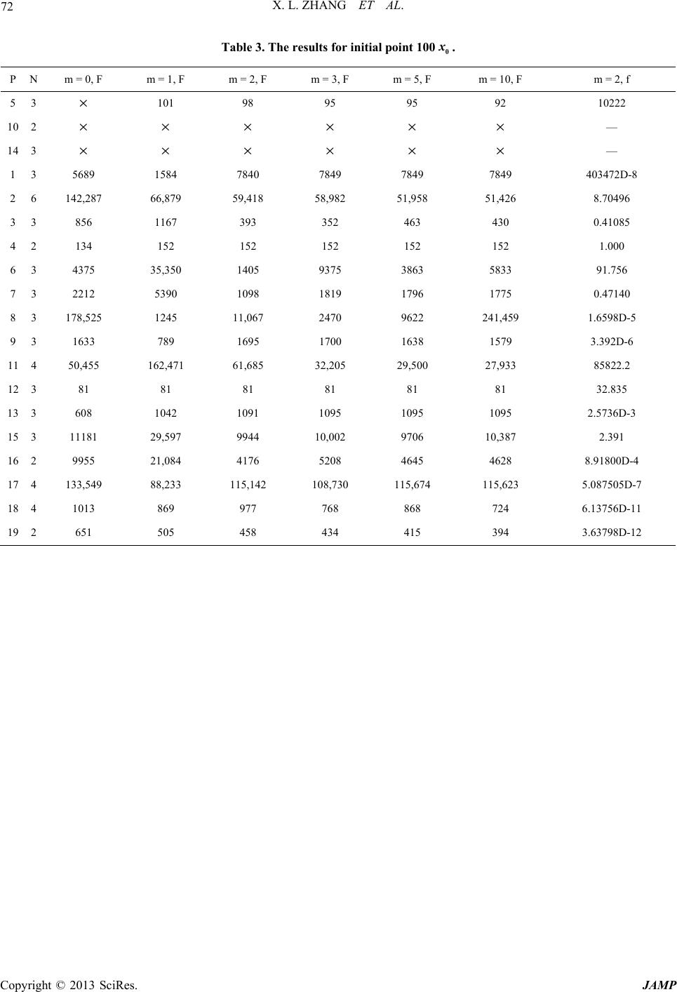 X. L. ZHANG ET AL. Copyright © 2013 SciRes. JAMP Table 3. The results for initial point 100 . P N m = 0, F m = 1, F m = 2, F m = 3, F m = 5, F m = 10, F m = 2, f 5 3 101 98 95 95 92 10222 10 2 — 14 3 — 1 3 5689 1584 7840 7849 7849 7849 403472D-8 2 6 142,287 66,879 59,418 58,982 51,958 51,426 8.70496 3 3 856 1167 393 352 463 430 0.41085 4 2 134 152 152 152 152 152 1.000 6 3 4375 35,350 1405 9375 3863 5833 91.756 7 3 2212 5390 1098 1819 1796 1775 0.47140 8 3 178,525 1245 11,067 2470 9622 241,459 1.6598D-5 9 3 1633 789 1695 1700 1638 1579 3.392D-6 11 4 50,455 162,471 61,685 32,205 29,500 27,933 85822.2 12 3 81 81 81 81 81 81 32.835 13 3 608 1042 1091 1095 1095 1095 2.5736D-3 15 3 11181 29,597 9944 10,002 9706 10,387 2.391 16 2 9955 21,084 4176 5208 4645 4628 8.91800D-4 17 4 133,549 88,233 115,142 108,730 115,674 115,623 5.087505D-7 18 4 1013 869 977 768 868 724 6.13756D-11 19 2 651 505 458 434 415 394 3.63798D-12
|