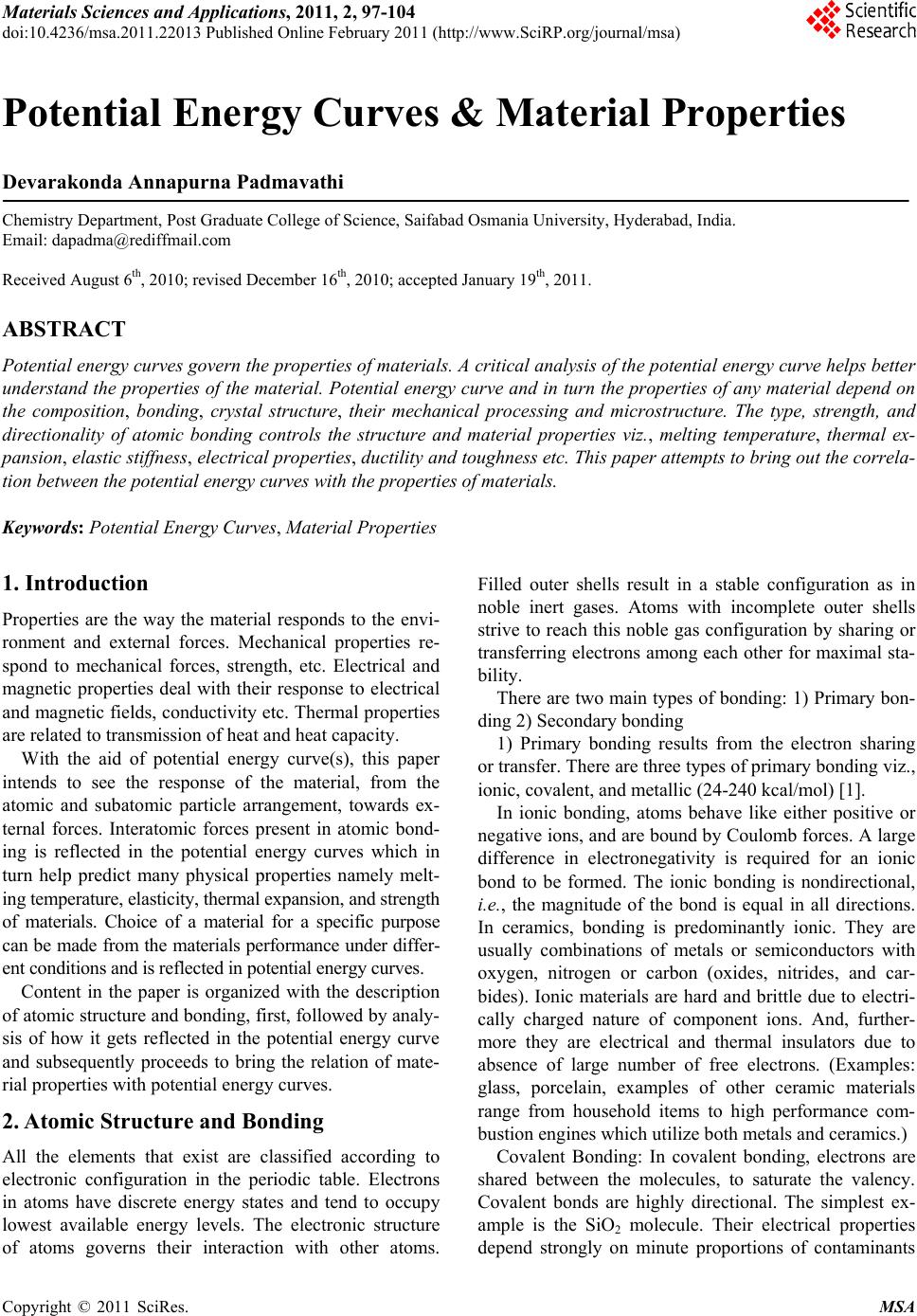Materials Sciences and Applicatio ns, 2011, 2, 97-104
doi:10.4236/msa.2011.22013 Published Online February 2011 (http://www.SciRP.org/journal/msa)
97
Potential Energy Curves & Material Properties
Devarakonda Annapurna Padmavathi
Chemistry Department, Post Graduate College of Science, Saifabad Osmania University, Hyderabad, India.
Received August 6th, 2010; revised December 16th, 2010; accepted January 19th, 2011.
ABSTRACT
Potential energy curves govern the properties of materials. A critical analysis of the potential energy curve helps better
understand the properties of the material. Potential energy curve and in turn the properties of any material depend on
the composition, bonding, crystal structure, their mechanical processing and microstructure. The type, strength, and
directionality of atomic bonding controls the structure and material properties viz., melting temperature, thermal ex-
pansion, elastic stiffness, electrical properties, ductility and toughness etc. This paper attempts to bring out the correla-
tion between the potential energy curves with the properties of materials.
Keywords: Potential Energy Curves, Material Properties
1. Introduction
Properties are the way the material responds to the envi-
ronment and external forces. Mechanical properties re-
spond to mechanical forces, strength, etc. Electrical and
magnetic properties deal with their response to electrical
and magnetic fields, conductivity etc. Thermal properties
are related to transmission of heat and heat capacity.
With the aid of potential energy curve(s), this paper
intends to see the response of the material, from the
atomic and subatomic particle arrangement, towards ex-
ternal forces. Interatomic forces present in atomic bond-
ing is reflected in the potential energy curves which in
turn help predict many physical properties namely melt-
ing temperature, elasticity, thermal expansion, and strength
of materials. Choice of a material for a specific purpose
can be made from the materials performance under differ-
ent conditions and is reflected in potential energy curves.
Content in the paper is organized with the description
of atomic structure and bonding, first, followed by analy-
sis of how it gets reflected in the potential energy curve
and subsequently proceeds to bring the relation of mate-
rial properties with potential energy curves.
2. Atomic Structure and Bonding
All the elements that exist are classified according to
electronic configuration in the periodic table. Electrons
in atoms have discrete energy states and tend to occupy
lowest available energy levels. The electronic structure
of atoms governs their interaction with other atoms.
Filled outer shells result in a stable configuration as in
noble inert gases. Atoms with incomplete outer shells
strive to reach this noble gas configuration by sharing or
transferring electrons among each other for maximal sta-
bility.
There are two main types of bonding: 1) Primary bon-
ding 2) Secondary bonding
1) Primary bonding results from the electron sharing
or transfer. There are three types of primary bonding viz.,
ionic, covalent, and metallic (24-240 kcal/mol) [1].
In ionic bonding, atoms behave like either positive or
negative ions, and are bound by Coulomb forces. A large
difference in electronegativity is required for an ionic
bond to be formed. The ionic bonding is nondirectional,
i.e., the magnitude of the bond is equal in all directions.
In ceramics, bonding is predominantly ionic. They are
usually combinations of metals or semiconductors with
oxygen, nitrogen or carbon (oxides, nitrides, and car-
bides). Ionic materials are hard and brittle due to electri-
cally charged nature of component ions. And, further-
more they are electrical and thermal insulators due to
absence of large number of free electrons. (Examples:
glass, porcelain, examples of other ceramic materials
range from household items to high performance com-
bustion engines which utilize both metals and ceramics.)
Covalent Bonding: In covalent bonding, electrons are
shared between the molecules, to saturate the valency.
Covalent bonds are highly directional. The simplest ex-
ample is the SiO2 molecule. Their electrical properties
depend strongly on minute proportions of contaminants

Potential Energy Curves & Material Properties
98
(Examples: Si, Ge, GaAs).
Metallic bonding: In metals, valence electrons are de-
tached from atoms, and spread in an ‘electron sea’ that
“glues” the ions together. Metals and alloys exhibit four
characteristic properties namely good ductility, high
thermal conductivity, high electrical conductivity and
metallic lustre due to their free electrons. Metallic bond-
ing is nondirectional and is rather insensitive to structure.
As a result high ductility is observed in metals where the
“bonds” do not “break” when atoms are rearranged –
examples of metals with typical metallic bonding: Cu, Al,
Au, Ag, etc. Transition metals (Fe, Ni, etc.) form mixed
bonds, comprising of metallic and covalent bonds in-
volving their 3d-electrons. As a result the transition met-
als are more brittle (less ductile) than Au or Cu.
2) Secondary bonding: There is no electron transfer or
sharing in secondary bonding. Secondary bonding also
called as van der Waals bonding, is much weaker as
compared to the primary bonding and results from inter-
action of atomic or molecular dipoles. Range of energy is
<24 kcal/mol.
Large difference in electronegativities between atoms,
result in asymmetrical arrangement of positively and
negatively charged regions (HCl, H2O) causing perma-
nent dipole moments. These polar molecules can induce
dipoles in adjacent non-polar molecules and bond is
formed due to the attraction between the permanent and
induced dipoles. Even in electrically symmetric mole-
cules/atoms (like H2, Cl2) an electric dipole can be in-
duced by fluctuations of electron density distribution.
Fluctuating electric field in one atom is felt by the elec-
trons of an adjacent atom, and induces a dipole momen-
tum in the other. This bond due to fluctuating induced
dipoles is the weakest (inert gases, H2, Cl2).
The strength of the secondary bonding depends on
strength of the dipole. Examples include permanent di-
poles (polar molecules—H2O, HCl...), fluctuating in-
duced dipoles (inert gases, H2, Cl2), dipole-induced
dipole bonds and induced dipole-induced dipole interac-
tions.
2.1. Bonding Forces and Energies
Physical properties are predicted based on interatomic
forces that bind the atoms together. Consider the
interaction of two isolated atoms as they are getting
closer from an infinite separation. At large distances
interactions are negligible but interactions grow up as
they approach each other. These forces are of two types
attractive force (FA) and repulsive force (FR) and the
magnitude of each is a function of interatomic distance.
The origin of the attractive part, depends on the particu-
lar type of bonding. The repulsion between atoms, when
they are brought close to each other, is related to the
Pauli principle: when the electronic clouds surrounding
the atoms start to overlap, the energy of the system in-
creases abruptly.
The net force F is sum of both attractive and repulsive
components. When FA and FR balance, or become equal,
there is no net force i.e., FA + FR = 0. Then a state of
equilibrium exists. This corresponsds to equilibrium
spacing as indicated in Figure 1. Sometimes it is more
convenient to work with potential energies between two
atoms instead of forces.
Mathematically energy (E) and force (F) are related as
EFd=r
∫
(1)
for atomic systems. At equilibrium spacing ro, net force is
zero and net energy corresponds to minimum energy Eo
[1]. When there are more than two atoms, force and
energy interactions among many atoms have to be consi-
dered. The minimum energy Eo is the binding energy
required to separate two atoms from their equilibrium
spacing to an infinite distance apart.
Figure 2 illustrates simple potential energy curves.
The energy Eo, shape and depth of the curve defines
various properties. The curves indicate the strength of the
bond based on the depth of the potential well. The more
deep the well, the more stable is the molecule, and a
shallower potential well indicates the molecule has low
Figure 1. A typical potential well indicating bonding
energies Eo and forces for two interacting atoms.

Potential Energy Curves & Material Properties99
Figure 2. Calculated quantum mechanical potential energy
curves of He2 and H2.
dissociation energy. The shallow potential energy curve
of helium states that the forces that bind are very weak.
Almost a zero Eo value indicates the instability of the
molecule. Very small bonding energy Eo of hydrogen
states that gaseous state is favored.
Table 1 gives list of bonding energies and melting
tenperatures for various bond types. Increase in depth of
the potential well, increases the melting temperature Tm
(Figure 3(b)). Molecules with large bonding energies
have high melting temperatures generally these exist as
solids. As the depth of the potential well decreases. the
molecules move from solid state to gaseous state [3].
3. Analysis of Potential Energy Curves
3.1. Packing of Crystal Structures and Their
Influence on Bonding Energies
Different atoms based on their nature, arrange them-
selves in different crystalline forms. The order in which
atoms associate with neighbors, determine the bonding
energy, the shape and depth of the potential well.
Table 1. Bonding energies and melting temperatures for
various substances.
Bonding Type Substance
Bonding
Energy
(kcal/mol)
Melting
Temperature
(˚C)
NaCl 153 801
Ionic
MgO 239 1000
Si 108 1410
C 170 > 3550 Covalent
Hg 16 –39
Al 77 660
Fe 97 1538 Metallic
W 203 3410
Ar 1.8 –189
vander Waals
Cl2 7.4 –101
(a)
(b)
Figure 3. (a) A typical potential energy curve; (b) Change in
shape of the well with temperature.

Potential Energy Curves & Material Properties
100
te, compress, twist) or
break as a function of applied load, time, temperature,
and other conditions is described by mechanical proper-
ties
Non-crystalline solids lack a systematic and regular
arrangement of atoms over relatively large atomic dis-
tances. This disordered or random packing of atoms
changes the force that binds the neighbouring atoms, and
hence the bonding energy Eo of neighbouring atoms is
different (Figure 4(a)). Due to the variation in neigh-
bouring bond lengths, materials density decreases which
has an influence on material properties.
In crystal structures with long range order atoms are
positioned in a repititive 3-dimensional
The standard language to discuss mechanical proper-
ties of materials is in terms of Hooke’s law. In this law,
stress ‘σ’ and strain ‘ε’ are related to each other by the
equation
E
σ
ε
=
(2)
where E is the modulus of Elasticity or Young’s Modulus
(Figure 6(a)).
pattern in which
each atom is bonded to its nearest neighbouring atoms
with similar force. As a result, equilibrium bond length ro
and bond energy Eo remains same between any two
neigbouring atoms (Figure 4(b)). And hence materials
with high ordered packing have good density and hence
good strength [2].
Different ordered packing results in different crystal-
line patterns. The
Hooke’s law allows one to compare specimens of dif-
ferent cross sectional area A0 and different length L0. This
equation can also be written in terms of force F as
0
o
F
L
E
A
L
Δ
= (3)
type of packing, nearest neighbour
bonding and crystal structure decide the properties of
substances. For ex., pure Mg hexagonal closely packed
crystal is more brittle than Al a face centered cubic crys-
tal due to less number of slip planes and hence undergoes
fracture at lower degrees of deformation (Figure 5).
3.2. Mechanical Properties
In the elastic limit Modulus of elasticity E is the slope
of the stress (F/A0) versus strain (ΔL/L0) curve (Figure
6(b)). Higher the modulus of elasticity higher is the
stiffness of the bond. After the stress is removed, if the
material returns to the dimension it had before the load-
ing, it is elastic deformation. If the material does not re-
turn to its previous dimension it is referred as plastic de-
formation.
On an atomic scale, macroscopic elastic strain is mani-
How materials deform (elonga
(a)
(b)
Figure 4. (a) Random packing of atoms and the corresping potential energy curve; (b) Dense orderedacking
of atoms and the corresponding potential energy curve.
ond p

Potential Energy Curves & Material Properties101
(a) (b) (c)
Figure 5. Packinracture. g of atoms in (a) Al, (b) Mg and (c) Relation between packing and f
(a)
(b)
Figure 6. (a) Variation of strwith strain; (b) Linearity of
stress strain relation.
ges in the interatomic spacing and
Modulus of eleasticity E is proportional to slope of the
(Figure 7(a))
at equilibrium spacing. Slope of the curve at r = r
es
n solids the principle mode of
s through increase in vibra-
ess
fested as small chan
the stretching of interatomic bonds. As a consequence,
the magnitude of modulus of elasticity is a measure of
the resistance to separation of adjacent atoms i.e., intera-
tomic bonding forces.
o
position is steep for very stiff materials and shallower for
flexible materials [2,3].
force versus interatomic separation curve
The energy interatomic distance curve, Figure 7(b)
illustrates that as modulus of elasticity E decreases, energy
minima decreases and hence the strength of the bond.
Values of modulus of eleasticity E are highest for cera-
mics, higher for metals and lower for polymers which is
a direct consequence of the different types of atomic
bonding.
Another measured mechanical property is yield strength.
This is the level of stress above which a material begins
to show permanent deformation. From an atomic pers-
pective, plastic deformation corresponds to the breaking
of bonds with original atom neighbors and then for-
mation of bonds with new ones as large number of
molecules move relative to one another. In plastic defor-
mation, upon removal of stress the atoms do not return to
their original positions.
Low yield strength corresponds to the inability of the
molecule to regain its initial state, which corresponds to
low elastic modulus and hence low bonding energy in the
potential energy curve.
Metals have high yield strength but for ceramics yield
strength is hard to measure, as since in tension fracture
occurs before it yields.
3.3. Thermal Properti
Response of a material to the application of heat is often
studied in terms of heat capacity, thermal expansion and
thermal conductivity. I
thermal energy assimilation i
tion energy of atoms. The vibrations of adjacent atoms
are coupled based on the nature of atomic bonding lead-
ing to lattice waves termed phonons which transfer en-
ergy through material.
Most solids expand on heating and contract on cooling.
Thermal expansion results in an increase in the average
distance between atoms. When the temperature changes,

Potential Energy Curves & Material Properties
102
(a)
(b)
Figure 7. (a) The force-distance curve for two materials,
showing the relationship between atomic bonding and the
modulus of elasticity, a steep dF/dr slope gives a high
modulus; (b) Potential curve with variation of inter atomic
distance and energy.
the amount by which a material changes its dimensions
in length, is given by linear coefficient of thermal expan-
sion ‘α’.
()
21
0
L
Linear coefficient of thermal expansion ‘α’ of the
material ca
LTT
α
=−
(4)
n be correlated with the shape of the curve.
The trough in the potential energy curve, corresponds to
the equilibrium interatomic spacing
Heating to successively higher temperatures (Figure
8(
by the mean
Δ
at 0 K.
a)) T1 to T5 raises the vibrational energy. At each tem-
perature, the width of the curve is proportional to the
amplitude of thermal vibrations for an atom, and the av-
erage interatomic distance is represented
(a)
(b)
Figure 8. (a) Variation of asymmetric potential energy
curve with Temperature T; (b) Variation of symmetric po-
tential energy curve with Temperature T.
position, which increases w temperature from r(T1) to
ith rising tem-
erature. The coefficient of thermal expansion ‘α’ is lar-
ith
r(T5). Thermal expansion is really due to the asymmetric
curvature of this potential energy trough, rather than the
increased atomic vibration amplitudes w
p
ger if Eo is smaller and the curve is very asymmetric.
If the potential energy curve were symmetric (Figure
8(b))
n α
in
is small, yielding a small α value.
Th
, there would be no net change in interatomic sepa-
ration with rise of temperature and, consequently, no
thermal expansion.
Magnitude of linear coefficient of thermal expansio
creases with increase in temperature. If inter-atomic
energy is large, and the well of potential curve is deep
and narrow the increase in inter atomic separation with
rise of temperature
is is observed in materials having strong bondng ener-
gies. When the material has small bond energies inter
atomic spacing increases with temperatue rise indicating
high thermal expansion α. (Figure 9). [2]

Potential Energy Curves & Material Properties103
Figure 9. The inter-atomic energy separation curve for two
atoms. Materials that display a steep curve with a deep
trough have low linear coefficients of thermal expansion.
Thermal conductivity values are lower for polymers,
in
olymers it is due to rotation and vibration of long chain
m
arameters which are geometry independent.
nductivity is strongly de-
ctrons available to partici-
nces each distinct
at
e 12(b) there is an overlap of
an
intermediate for ceramics and maximum for metals. This
is because in metals the vibration transfer is through at-
oms and electrons, in ceramics it is through atoms and
p
olecules.
3.4. Electrical Properties
Solid materials exhibit a very wide range of electrical
conductivity [1,3]. Electrical conductivity and resistivity
are material p
The magnitude of electrical co
pendent on the number of ele
pate in the conduction process.
Consider a solid of N atoms. Initially, at relatively
large separation distances, each atom is independent of
its neighbors. However as the atoms approach close with
one another electrons of one atom are perturbed by elec-
tron and nuclei of another. This influe
omic state to split into a series of closely spaced elec-
tronic levels in the solid termed as an electron energy
band (Figure 10). Large numbers of individual energy
levels overlap and form a band (Figure 11). The number
of states within each band equals the total of all states
contributed by the N atoms. Within each band, the en-
ergy states are discrete, yet the difference between adja-
cent states is exceedingly small. Furthermore, gaps may
exist in the adjacent bands.
Four different types of band structures are possible at 0
K. In Figure 12(a) the outermost band is only partially
filled with electrons. This type of band structure is seen
in metals with a single s valence electron. For the sec-
ond band structure in Figur
empty band and a filled band. In the last two band
structures Figure 12(c) and Figure 12(d) the band com-
pletely filled with electrons is separated from an empty
conduction band. The magnitude of energy gap is the
Figure 10. The energy levels broaden into bands as the
number of electrons grouped together increases.
Figure 11. Energy band structure in solids.
(a) (b) (c) (d)
Figure 12. The various possible electron band structures in
solids at 0 K: (a) Metals such as copper, in which electron
states are available above and adjacent to filled states, in
the same band; (b) The electron band structure of metal
such illed
and empty outer bands; (c) Insulators: the filled va
emiconductors, and insulators have dif-
rent accessibility to energy states for conductance of
s
as magnesium, wherein there is an overlap of f
lence
band is separated from the empty conduction band by a
relatively large band gap (>2 eV); (d) Semiconductors:
same as for insulators except that the band gap is relatively
narrow (<2 eV).
only difference between the two band structures, for ma-
terials that are insulators the band gap is wide whereas
for semiconductors it is narrow [1].
Conductors, s
fe

Potential Energy Curves & Material Properties
104
ve very low conduc-
tiv
curve indicates large bond
emperature, large elastic modulus
t of thermal expansion.
different
m
nd small coefficient of linear expansion
fo
tial energy curves of metals possess variable
bo
an
pansion. Polymers possessing directional prop-
ert
ion exists for solid materials as
in
covalent and ionic in semi-
co
gineering: An
Introduction,” & Sons, Inc., Ho-
boken, 2008.
rove, 2003.
electrons. Metallic conductivity is of the order of 107
(Ω-m)–1, semiconductors have intermediate conductivities
10–6 to 104 (Ω-m)–1 and insulators ha
ities 10–10 to 10–20 (Ω-m)–1.
4. Conclusions
The magnitude of bonding energy and shape of the po-
tential energy curve varies from material to material. A
deep and narrow trough in the
energy, high melting t
and small coefficien
Generally substances with large bonding energy Eo are
solids, intermediate energies are liquids and small ener-
gies are gases.
The width and asymmetry of the well in the potential
energy curve represents varying properties of
aterials.
Large bond energies, high melting temperature, large
elastic modulus a
und in potential energy curve(s) of ceramics represent
very good strength, characteristically hard nature.
The poten
nd energy, reasonably high melting point, high elastic
modulus, and moderate thermal expansion. The ductility
of metals is implicitly related to the characteristics of the
metallic bond. The grouping of energy levels as bands [3] W. F. Smith, “Principles of Materials Science and Engi-
neering,” 3rd Edition, McGraw-Hill, Columbus, 1996.
d their overlap with availability of large number of free
electrons is responsible for electrical conductivity of
metals.
The potential curve(s) of polymers possess low melt-
ing point low elastic modulus and large coefficient of
linear ex
ies due to covalent bonding have dominating second-
dary forces of interactions and influence the physical
properties of materials.
This paper focused on an ideal situation involving only
two atoms to understand some of the properties, a similar
yet more complex condit
teractions among many atoms need to be addressed.
However, the energy versus interatomic separation curve
defines the basic property.
In many materials more than one type of bonding is
involved viz., ionic and covalent in ceramics, covalent
and secondary in polymers,
nductors. These are to be considered while deriving the
properties from the potential energy curves.
REFERENCES
[1] W. D. Callister, “Materials Science & En
7th Edition, John Wiley
[2] D. R. Askeland and P. P. Phule. “The Science and Engi-
neering of Materials,” 4th Edition, Thomas Book Com-
pany, Pacific G