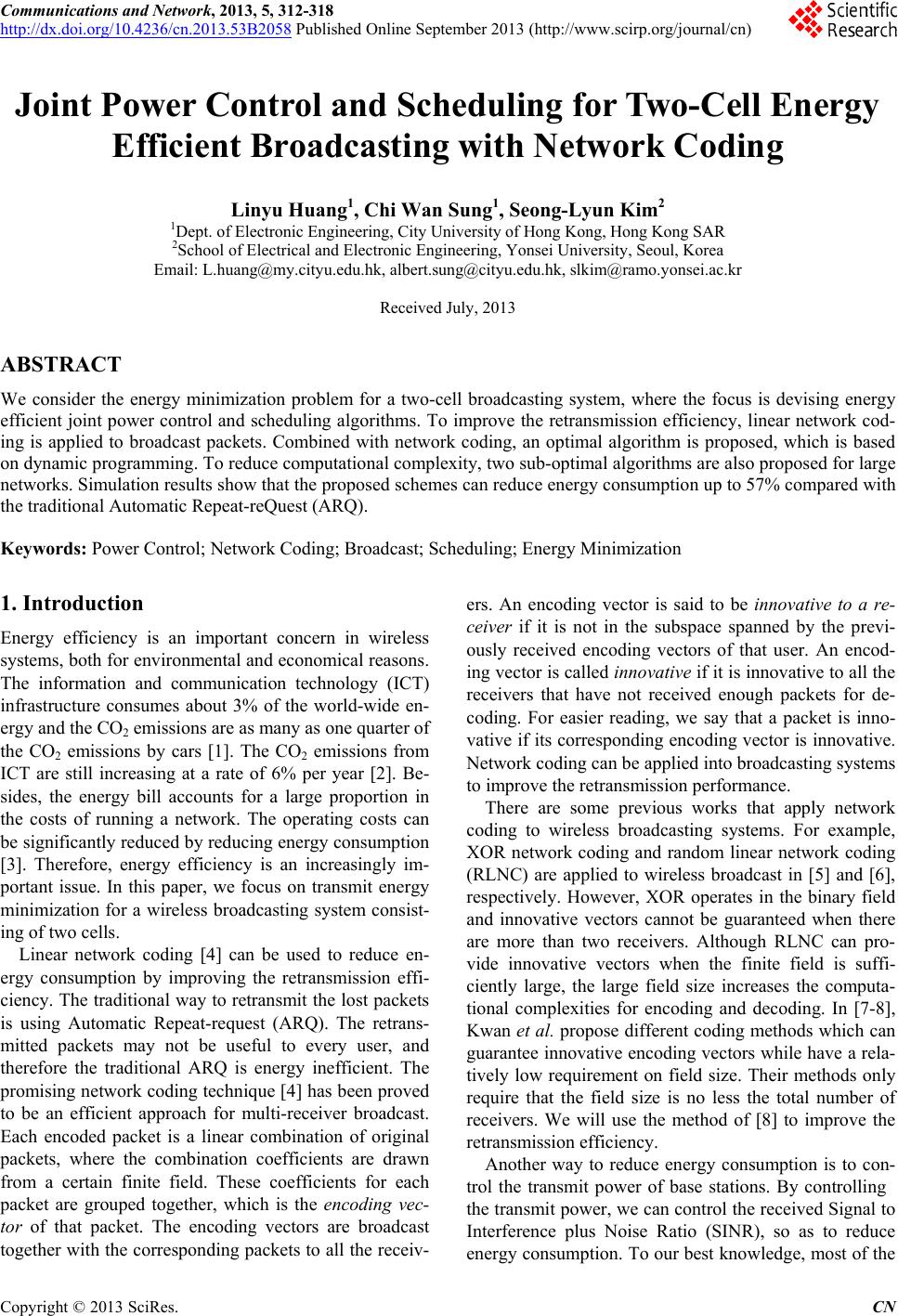Communications and Network, 2013, 5, 312-318
http://dx.doi.org/10.4236/cn.2013.53B2058 Published Online September 2013 (http://www.scirp.org/journal/cn)
Joint Power Control and Scheduling for Two-Cell Energy
Efficient Broadcasting with Network Coding
Linyu Huang1, Chi Wan Sung1, Seong-Lyun Kim2
1Dept. of Electronic Engineering, City University of Hong Kong, Hong Kong SAR
2School of Electrical and Electronic Engineering, Yonsei University, Seoul, Korea
Received July, 2013
ABSTRACT
We consider the energy minimization problem for a two-cell broadcasting system, where the focus is devising energy
efficient joint power control and scheduling algorithms. To improve the retransmission efficiency, linear network cod-
ing is applied to broadcast packets. Combined with network coding, an optimal algorithm is proposed, which is based
on dynamic programming. To reduce computational complexity, two sub-optimal algorithms are also proposed for large
networks. Simulation results show that the proposed schemes can reduce energy consumption up to 57% compared with
the traditional Automatic Repeat-reQuest (ARQ).
Keywords: Power Control; Network Coding; Broadcast; Scheduling; Energy Minimization
1. Introduction
Energy efficiency is an important concern in wireless
systems, both for environmental and economical reasons.
The information and communication technology (ICT)
infrastructure consumes about 3% of the world-wide en-
ergy and the CO2 emissions are as many as one quarter of
the CO2 emissions by cars [1]. The CO2 emissions from
ICT are still increasing at a rate of 6% per year [2]. Be-
sides, the energy bill accounts for a large proportion in
the costs of running a network. The operating costs can
be significantly reduced by reducing energy consumption
[3]. Therefore, energy efficiency is an increasingly im-
portant issue. In this paper, we focus on transmit energy
minimization for a wireless broadcasting system consist-
ing of two cells.
Linear network coding [4] can be used to reduce en-
ergy consumption by improving the retransmission effi-
ciency. The traditional way to retransmit the lost packets
is using Automatic Repeat-request (ARQ). The retrans-
mitted packets may not be useful to every user, and
therefore the traditional ARQ is energy inefficient. The
promising network coding technique [4] has been proved
to be an efficient approach for multi-receiver broadcast.
Each encoded packet is a linear combination of original
packets, where the combination coefficients are drawn
from a certain finite field. These coefficients for each
packet are grouped together, which is the encoding vec-
tor of that packet. The encoding vectors are broadcast
together with the corresponding packets to all the receiv-
ers. An encoding vector is said to be innovative to a re-
ceiver if it is not in the subspace spanned by the previ-
ously received encoding vectors of that user. An encod-
ing vector is called innovative if it is innovative to all the
receivers that have not received enough packets for de-
coding. For easier reading, we say that a packet is inno-
vative if its corresponding encoding vector is innovative.
Network coding can be applied into broadcasting systems
to improve the retransmission performance.
There are some previous works that apply network
coding to wireless broadcasting systems. For example,
XOR network coding and random linear network coding
(RLNC) are applied to wireless broadcast in [5] and [6],
respectively. However, XOR operates in the binary field
and innovative vectors cannot be guaranteed when there
are more than two receivers. Although RLNC can pro-
vide innovative vectors when the finite field is suffi-
ciently large, the large field size increases the computa-
tional complexities for encoding and decoding. In [7-8],
Kwan et al. propose different coding methods which can
guarantee innovative encoding vectors while have a rela-
tively low requirement on field size. Their methods only
require that the field size is no less the total number of
receivers. We will use the method of [8] to improve the
retransmission efficiency.
Another way to reduce energy consumption is to con-
trol the transmit power of base stations. By controlling
the transmit power, we can control the received Signal to
Interference plus Noise Ratio (SINR), so as to reduce
energy consumption. To our best knowledge, most of the

L. Y. HUANG ET AL.
313
previous works on energy minimization for broadcasting
are based on power control only [9] (and the references
therein) [10], without using network coding. Although
Tran et al. consider both power control and network
coding in [5], their network coding method works over
GF(2) which cannot guarantee that all the encoding vec-
tors are innovative. Note that both our power control
scheme and network coding method are different from
those in [5].
In this paper, we combine power control together with
network coding for broadcasting networks. We focus on
the joint power control and scheduling problem for two
base stations. The objective is to minimize the expected
transmit energy consumption. We use the network cod-
ing method proposed in [8] to generate innovative pack-
ets for transmissions. Combined with network coding, we
propose three joint power control and scheduling algo-
rithms to minimize energy consumption. In the first algo-
rithm, the problem is formulated as a dynamic program-
ming problem, which can provide an optimal solution, in
the sense of minimizing the expected energy consump-
tion. To reduce the computational complexity, two heu-
ristic algorithms are also proposed for large networks.
Simulation shows that they perform very well.
2. System Model
As shown in Figure 1, we consider a time slotted wire-
less broadcast system consisting of two partially over-
lapped cells and K users. The two base stations are de-
noted by BS1 and BS2, respectively. The transmission
range of each base station is a circle with radius r. The
distance between the two base stations is denoted by D.
We define a parameter δ = D/r, where 0 < δ < 2, to char-
acterize the locations of the two cells. The K users are
randomly located in the two cells and labeled as Ui,
where i∈{1, 2, …, K}. The distance from BSb, where b
∈{1, 2}, to user Ui is denoted by dbi. A broadcast file is
divided into N equal-size packets which are called un-
coded packets. Both BS1 and BS2 have all the N uncoded
packets. They want to broadcast these N packets to all the
K users by cooperating with each other.
Figure 1. System model.
Both BS1 and BS2 can transmit to the users in their own
transmission range. To avoid collisions, they are not al-
lowed to transmit simultaneously. At each time slot, both
BS1 and BS2 can change its transmit power to a value
which is chosen from a preset power level collection ϴ =
{θ1, θ2, …, θ| ϴ |,} (in mW units). All downlink channels
are modeled as mutually independent channels, across
time and across users, which are affected by path loss
and Rayleigh fading. A packet is considered to be suc-
cessfully received if the received SINR is greater than a
predetermined threshold Γ (in dB units). Otherwise, that
packet will be considered to be lost. We use Rbi(θm) to
denote the reliability of the downlink channel from BSb
to user Ui with transmit power θm. The reliability is de-
fined as the probability that the received SINR is greater
than the threshold Γ. Since the received signal is subject
to Rayleigh fading, the instantaneous SINR is distributed
according to an exponential distribution with parameter
1/ASE A [11], where ASE A is the average SINR. According to
the cumulative distribution function of exponential dis-
tribution, the reliability Rbi(θm) can be computed by

{} exp(),
bi mr
RPS S 


(1)
where Sr is the instantaneous received SINR and ASE A is
the average SINR (in dB units). Note that ASE A is deter-
mined by the corresponding distance dbi and transmit
power θm. Depending on the environment, ASE Acan be ob-
tained by using the corresponding radio propagation
model, such as the Okumura model and Hata model.
Once a user successfully received a packet, it will send
an acknowledgement to the sender of that packet. All the
acknowledgement channels are assumed to be reliable
channels without error and delay. BS1 and BS2 are also
assumed to be connected via a wired cable and they can
share the acknowledgement information with each other.
All the packets transmitted by the base stations are
coded packets based on linear network coding. We as-
sume that the coding is operated over a finite field with q
elements, GF(q), where q ≥ K. We use the network cod-
ing method proposed in [8]. Since q ≥ K, it is guaranteed
that each broadcast packet is innovative to all users. In
other words, a user can recover the original file as long
as it has successfully received any N broadcast packets.
An example of network coding is given in Example 1.
For more details about the network coding method, we
refer the reader to [8]. We say that Ui is complete if it has
received N broadcast packets. Otherwise, we say that Ui
is incomplete.
Example 1: Let q = 3, K = 3 and N = 3. We assume
that each encoding vector is a 1×3 row vector. For exam-
ple, an encoding vector [1 0 1] means that the corre-
sponding encoded packet is obtained by taking linear
combinations of the first and the third uncoded packets

L. Y. HUANG ET AL.
314
with coefficients being 1.
Let Ci be the encoding matrix of user Ui, where its
rows represent the encoding vectors Ui has received so
far. At a particular time slot, consider
12 3
010 001100
,
101 110011
CCandC
 
 
 
 
Each user needs to receive at least one more packet for
successfully decoding the original file. If the network
coding method proposed in [8] is used, we can broadcast
an encoding vector v* = [0 1 2] to all users in one time
slot. For each Ui, v* is not in the row space of Ci, i.e. v*
cannot be obtained by taking linear combinations of row
vectors in Ci over GF(3). Therefore, v* is innovative to
all the three users. As long as Ui can successfully receive
v*, it can get a full rank matrix by appending v* to the
end of Ci. Then, Ui can successfully decode the original
file by using Gaussian elimination to solve the matrix
equations.
However, if XOR network coding is used, it cannot
find such an encoding vector that is innovative to all the
three users simultaneously. It requires at least two trans-
missions. For example, the base station may transmit the
encoding vector [0 1 1] to U1 and U2 in the first slot and
the encoding vector [0 1 0] to U3 in the second slot. The
network coding method proposed in [8] outweighs XOR
in this case.
Given a scheduling scheme B, we use an integer ran-
dom variable TB to denote the required number of trans-
missions for B to complete the broadcast. We define the
broadcast schedule of B as a binary sequence, ΦB = { ϕ
1,
ϕ
2, …,
ϕ
TB }. If
ϕ
t = 0, BS1 is selected to transmit at the
t-th time slot. Otherwise, if ϕ
t = 1, BS2 is selected. We
define the sequence of transmit power ΛB as{λ1, λ2, …,
λTB}, where λt∈ϴ is the transmit power level used at the
t-th time slot.
At time t, B specifies a function ft to determine ϕ
t and
λt:
1112 22111
(,)(,, ,,,,,,,)
ttttt t
f

 

ee e
where et is the channel status at the t-th time slot. It is a
binary random vector of length K. If et(i) = 1, it means
that the channel between the transmitter and Ui is too bad
and Ui cannot receive the broadcast packet. Otherwise, Ui
can receive that packet. Note that the probability distri-
bution of et depends on whether BS1 or BS2 is chosen as
the transmitter at time t. We call a realization of the se-
quence {e1, e2, …, eTB} a channel realization under B,
denoted by ΩB.
For a transmission with transmit power λt, the energy
consumption is λt times the duration of a time slot. To
simplify notations, we assume that the duration is one
unit and will be ignored throughout this paper. Therefore,
the total energy consumption of a particular channel re-
alization ΩB is denoted by XB and can be computed as
1
.
T
t
t
X

B
B

The expected energy consumption of B is denoted by
E[XB], where the expectation is taken with respect to the
probability distribution of et, which depends on ϕ
t. Our
objective is to minimize E[XB] by determining an optimal
scheduling scheme B which requires to determine ΦB and
ΛB as well.
3. Optimal Scheme
The joint power control and scheduling problem can be
formulated as a dynamic programming problem with the
following parameters.
 State We define the state of all users as a 1×K state
vector s = [s1 s2 … sK], where si, 0 < i ≤ K, denotes the
number of packets that Ui has received. The state space is
denoted by S = [ s1 s2 … sK], where 0 ≤ si ≤ N and 0 <
i ≤ K. The goal state is defined as sg = [N N … N], which
means every user has received N packets and can be con-
sidered as a complete user.
 Action At each time step, we need to determine
both the transmitter and the transmit power. We define
the action set as A = {0, 1} × ϴ. At each time slot, an
action a = (b, θ) is selected from A. Action a = (b, θm)
means that BSb is selected to transmit with transmit
power θm.
 State Transition Probability Given a state s, let
p(s'|s, a) denote the state transition probability that trans-
fers from s to s' under action a. Now, we are going to
introduce how to compute the state transition probability
p(s'|s, a).
For a given action a = (b, θm) and given states s = [s1
s2 … sK] and s' = [s1' s2' … sK'], we use p(si'|si, a) to de-
note the probability that the number of packets received
by Ui changes from si to si' under action a. Since all the
downlink channels are assumed to be mutually inde-
pendent across users, the state transition probability p(s'|s,
a) is the product of p(si'|si, a) for all users. Hence,
1
('|, )( '|,)
K
ii
i
p
apssass


We define Qi(a) as the success probability of taking
action a to transmit to user Ui. Based on the previous dis-
cussion, Qi(a) equals the reliability Rbi(θm) and Qi(a) can
be obtained by Equation (1). Based on the given states s,
s' and the number of packets that Ui has received, the
state transition for Ui can be classified into five different
cases. The transition probability of each case can be ob-
tained by the following equation.

L. Y. HUANG ET AL.
315
0,' ,
1,' ,
('|,) 1(),',
(),' 1,
0,' 2.
ii
ii
iiiii
iii
ii
ss
s
sN
pssaQ assN
Qas s
ss
if
if
if
if
if





 





Now we are going to discuss how to find the optimal
action for each state. For s∈S, we define V(s) as the ex-
pected energy consumption for the system to evolve from
s to sg given that optimal actions are chosen in every state,
and define π(s) as the optimal action at state s. It is clear
that V(s) is non-zero except when s = sg. For s∈S \ {sg},
we define V(s, a) as the expected energy consumption for
the system to evolve from s to sg given that action a is
chosen for state s and optimal actions are chosen for the
other states. For a given action a = (b, θm) ∈A, V(s, a)
can be computed by solving the following equation:
'{}
(,)('| ,)(')( | ,)(,),
m
VapaVpaVa 
sS\s
sssssss

 
 (2)
where θm means that each state transition takes one
transmission and θm is the energy consumption of that
transmission. Note that the summation only involves
those states that can be immediately reached from s. In
other words, state s' is involved only when p(s'|s, a) is
non-zero. Equation (2) can be written as:
'{}
(,)[( '|,)(')]/[1(|,)]
m
VapaVp a 
sS\s
ssssss

 
 (3)
Note that our problem has the property that the
state-transition graph is a directed acyclic graph. It
mea-ns that given two distinct states, s and s', if s' can be
reached from s after a certain number of state transitions,
then s cannot be reached from s'. Figure 2 shows an ex-
ample of the state transition graph for K = 2 and N = 2.
For directed acyclic graph, it is well known that there is a
topological ordering of vertices, which means that if
there is a state transition from s to s', then s comes before
s' in the ordering. Due to this property, V(s) can be com-
puted backward from V(sg). To compute V(s), we apply
the formula in (3) to find V(s, a). V(s) and the optimal
action at s can then be obtained by
Figure 2. State-transition graph for K=2 and N=2.
Algorithm 1: Dynamic Programming (DP) Algorithm
Input: The initial state s=01×K
Output: V(s) and π(s) for all s∈S
set V(s):=0 and π(s):= 0 for all s∈S //global vari-
ables
do OptimalAction(s)
return V(s) and π(s) for all s∈S
Function: OptimalAction(s)
for s'∈S \ {sg, s} do
if p(s'|s, a) > 0 for any a∈A and V(s')=0
do OptimalAction(s')
end if
end for
for a = (b,θm) ∈A do
'{}
(,):[('| ,)(')]/[1(| ,)]
m
VapaVp a 

 

sS\s
ssssss
end for
(): min(, )
π(): argmin(,)
a
a
VVa
Va




A
A
ss
ss
end function
()min(, )()argmin(, ),
aa
VVa Va
AA
ssandπss



respectively. To implement this idea, recursion may be
used, and we state the recursive algorithm in Algorithm
(1). We call it Dynamic Programming (DP) scheme.
By the principle of optimality [12], DP is optimal in
terms of minimizing expected energy consumption.
4. Heuristic Schemes
While DP is optimal, its time complexity grows expo-
nentially with K. To reduce complexity, we propose two
fast heuristic algorithms for large networks. When the
number of users is relatively small, we propose a greedy
algorithm which dynamically changes the transmit power.
When the number of users is very large, we propose an
algorithm which uses fixed transmit power.
4.1. Greedy Algorithm
The greedy algorithm has the following three steps.
Step 1: At the beginning of a time slot, let sj, where 0
< j ≤ K, denote the number of packets that Uj has re-
ceived. We first choose the user Ui which has received
the least number of packets. If there are multiple quali-
fied users, we will randomly pick one of them.
Step 2: Select the base station BSb* that is closer to Ui
as the sender. If both BS1 and BS2 have the same distance
from Ui, randomly pick one of them as the sender in the
current slot.
Step 3: We define a parameter Ebi(θm) for each trans-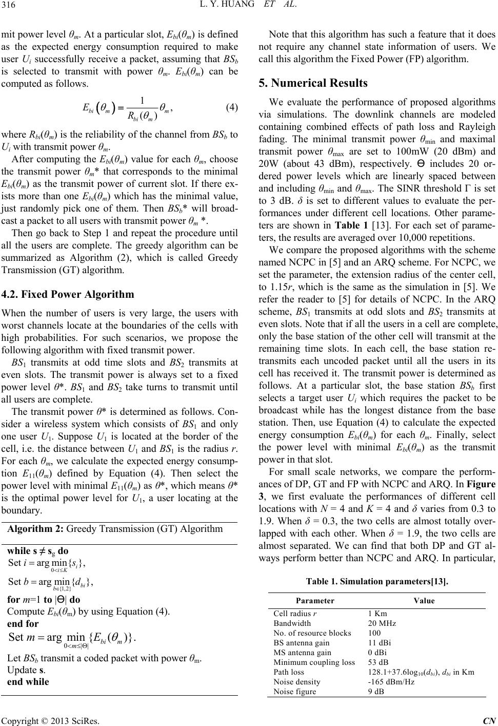

L. Y. HUANG ET AL.
316
mit power level θm. At a particular slot, Ebi(θm) is defined
as the expected energy consumption required to make
user Ui successfully receive a packet, assuming that BSb
is selected to transmit with power θm. Ebi(θm) can be
computed as follows.

1,
()
bi mm
bi m
ER



 (4)
where Rbi(θm) is the reliability of the channel from BSb to
Ui with transmit power θm.
After computing the Ebi(θm) value for each θm, choose
the transmit power θm* that corresponds to the minimal
Ebi(θm) as the transmit power of current slot. If there ex-
ists more than one Ebi(θm) which has the minimal value,
just randomly pick one of them. Then BSb* will broad-
cast a packet to all users with transmit power θm *.
Then go back to Step 1 and repeat the procedure until
all the users are complete. The greedy algorithm can be
summarized as Algorithm (2), which is called Greedy
Transmission (GT) algorithm.
4.2. Fixed Power Algorithm
When the number of users is very large, the users with
worst channels locate at the boundaries of the cells with
high probabilities. For such scenarios, we propose the
following algorithm with fixed transmit power.
BS1 transmits at odd time slots and BS2 transmits at
even slots. The transmit power is always set to a fixed
power level θ*. BS 1 and BS2 take turns to transmit until
all users are complete.
The transmit power θ* is determined as follows. Con-
sider a wireless system which consists of BS1 and only
one user U1. Suppose U1 is located at the border of the
cell, i.e. the distance between U1 and BS1 is the radius r.
For each θm, we calculate the expected energy consump-
tion E11(θm) defined by Equation (4). Then select the
power level with minimal E11(θm) as θ*, which means θ*
is the optimal power level for U1, a user locating at the
boundary.
Algorithm 2: Greedy Transmission (GT) Algorithm
while s ≠ sg do
0
{1, 2 }
Set argmin{},
Set argmin{},
i
iK
bi
b
is
bd




for m=1 to |ϴ| do
Compute Ebi(θm) by using Equation (4).
end for
0||
Set argmin{()}.
bi m
m
mE



Let BSb transmit a coded packet with power θm.
Update s.
end while
Note that this algorithm has such a feature that it does
not require any channel state information of users. We
call this algorithm the Fixed Power (FP) algorithm.
5. Numerical Results
We evaluate the performance of proposed algorithms
via simulations. The downlink channels are modeled
containing combined effects of path loss and Rayleigh
fading. The minimal transmit power θmin and maximal
transmit power θmax are set to 100mW (20 dBm) and
20W (about 43 dBm), respectively. ϴ includes 20 or-
dered power levels which are linearly spaced between
and including θmin and θmax. The SINR threshold Γ is set
to 3 dB. δ is set to different values to evaluate the per-
formances under different cell locations. Other parame-
ters are shown in Table 1 [13]. For each set of parame-
ters, the results are averaged over 10,000 repetitions.
We compare the proposed algorithms with the scheme
named NCPC in [5] and an ARQ scheme. For NCPC, we
set the parameter, the extension radius of the center cell,
to 1.15r, which is the same as the simulation in [5]. We
refer the reader to [5] for details of NCPC. In the ARQ
scheme, BS1 transmits at odd slots and BS2 transmits at
even slots. Note that if all the users in a cell are complete,
only the base station of the other cell will transmit at the
remaining time slots. In each cell, the base station re-
transmits each uncoded packet until all the users in its
cell has received it. The transmit power is determined as
follows. At a particular slot, the base station BSb first
selects a target user Ui which requires the packet to be
broadcast while has the longest distance from the base
station. Then, use Equation (4) to calculate the expected
energy consumption Ebi(θm) for each θm. Finally, select
the power level with minimal Ebi(θm) as the transmit
power in that slot.
For small scale networks, we compare the perform-
ances of DP, GT and FP with NCPC and ARQ. In Figure
3, we first evaluate the performances of different cell
locations with N = 4 and K = 4 and δ varies from 0.3 to
1.9. When δ = 0.3, the two cells are almost totally over-
lapped with each other. When δ = 1.9, the two cells are
almost separated. We can find that both DP and GT al-
ways perform better than NCPC and ARQ. In particular,
Table 1. Simulation parameters[13].
Parameter Value
Cell radius r 1 Km
Bandwidth 20 MHz
No. of resource blocks 100
BS antenna gain 11 dBi
MS antenna gain 0 dBi
Minimum coupling loss53 dB
Path loss 128.1+37.6log10(dbi), dbi in Km
Noise density -165 dBm/Hz
Noise figure 9 dB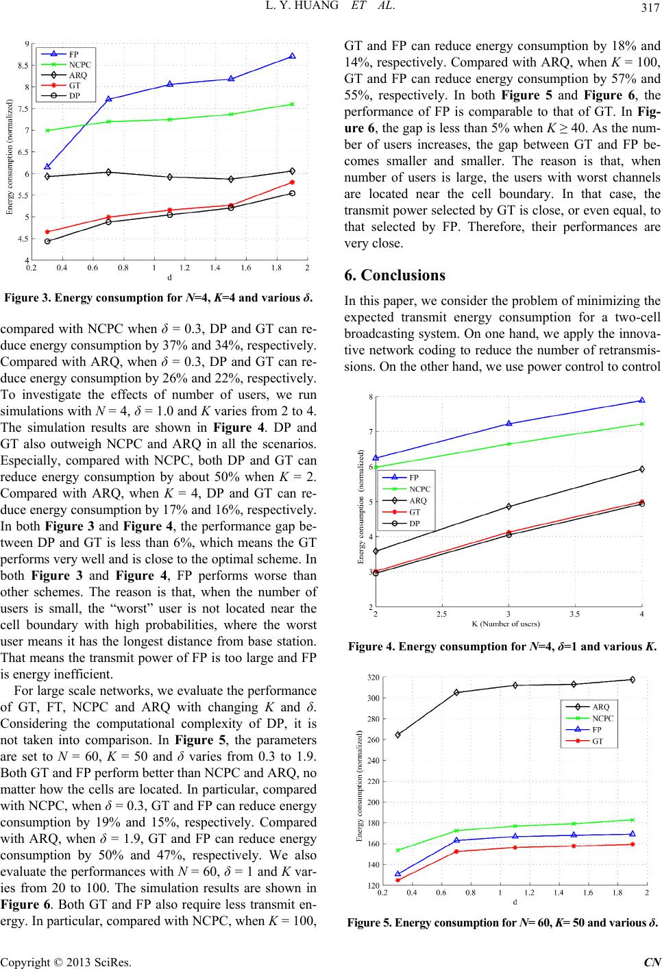

L. Y. HUANG ET AL.
317
Figure 3. Energy consumption for N=4, K=4 and various δ.
compared with NCPC when δ = 0.3, DP and GT can re-
duce energy consumption by 37% and 34%, respectively.
Compared with ARQ, when δ = 0.3, DP and GT can re-
duce energy consumption by 26% and 22%, respectively.
To investigate the effects of number of users, we run
simulations with N = 4, δ = 1.0 and K varies from 2 to 4.
The simulation results are shown in Figure 4. DP and
GT also outweigh NCPC and ARQ in all the scenarios.
Especially, compared with NCPC, both DP and GT can
reduce energy consumption by about 50% when K = 2.
Compared with ARQ, when K = 4, DP and GT can re-
duce energy consumption by 17% and 16%, respectively.
In both Figure 3 and Figure 4, the performance gap be-
tween DP and GT is less than 6%, which means the GT
performs very well and is close to the optimal scheme. In
both Figure 3 and Figure 4, FP performs worse than
other schemes. The reason is that, when the number of
users is small, the “worst” user is not located near the
cell boundary with high probabilities, where the worst
user means it has the longest distance from base station.
That means the transmit power of FP is too large and FP
is energy inefficient.
For large scale networks, we evaluate the performance
of GT, FT, NCPC and ARQ with changing K and δ.
Considering the computational complexity of DP, it is
not taken into comparison. In Figure 5, the parameters
are set to N = 60, K = 50 and δ varies from 0.3 to 1.9.
Both GT and FP perform better than NCPC and ARQ, no
matter how the cells are located. In particular, compared
with NCPC, when δ = 0.3, GT and FP can reduce energy
consumption by 19% and 15%, respectively. Compared
with ARQ, when δ = 1.9, GT and FP can reduce energy
consumption by 50% and 47%, respectively. We also
evaluate the performances with N = 60, δ = 1 and K var-
ies from 20 to 100. The simulation results are shown in
Figure 6. Both GT and FP also require less transmit en-
ergy. In particular, compared with NCPC, when K = 100,
GT and FP can reduce energy consumption by 18% and
14%, respectively. Compared with ARQ, when K = 100,
GT and FP can reduce energy consumption by 57% and
55%, respectively. In both Figure 5 and Figure 6, the
performance of FP is comparable to that of GT. In Fig-
ure 6, the gap is less than 5% when K ≥ 40. As the num-
ber of users increases, the gap between GT and FP be-
comes smaller and smaller. The reason is that, when
number of users is large, the users with worst channels
are located near the cell boundary. In that case, the
transmit power selected by GT is close, or even equal, to
that selected by FP. Therefore, their performances are
very close.
6. Conclusions
In this paper, we consider the problem of minimizing the
expected transmit energy consumption for a two-cell
broadcasting system. On one hand, we apply the innova-
tive network coding to reduce the number of retransmis-
sions. On the other hand, we use power control to control
Figure 4. Energy consumption for N=4, δ=1 and various K.
Figure 5. Energy consumption for N= 60, K= 50 and various δ.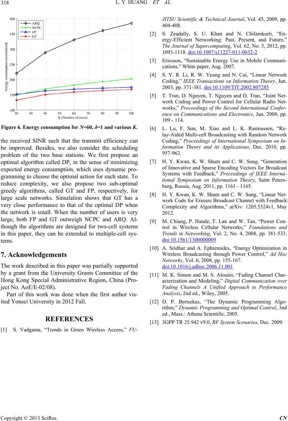

L. Y. HUANG ET AL.
318
Figure 6. Energy consumption for N=60, δ=1 and various K.
the received SINR such that the transmit efficiency can
be improved. Besides, we also consider the scheduling
problem of the two base stations. We first propose an
optimal algorithm called DP, in the sense of minimizing
expected energy consumption, which uses dynamic pro-
gramming to choose the optimal action for each state. To
reduce complexity, we also propose two sub-optimal
greedy algorithms, called GT and FP, respectively, for
large scale networks. Simulation shows that GT has a
very close performance to that of the optimal DP when
the network is small. When the number of users is very
large, both FP and GT outweigh NCPC and ARQ. Al-
though the algorithms are designed for two-cell systems
in this paper, they can be extended to multiple-cell sys-
tems.
7. Acknowledgements
The work described in this paper was partially supported
by a grant from the University Grants Committee of the
Hong Kong Special Administrative Region, China (Pro-
ject No. AoE/E-02/08).
Part of this work was done when the first author vis-
ited Yonsei University in 2012 Fall.
REFERENCES
[1] S. Vadgama, “Trends in Green Wireless Access,” FU-
JITSU Scientific & Technical Journal, Vol. 45, 2009, pp.
404-408.
[2] S. Zeadally, S. U. Khan and N. Chilamkurti, “En-
ergy-Efficient Networking: Past, Present, and Future,”
The Journal of Supercomputing, Vol. 62, No. 3, 2012, pp.
1093-1118. HUdoi:10.1007/s11227-011-0632-2UH
[3] Ericsson, “Sustainable Energy Use in Mobile Communi-
cations,” White paper, Aug. 2007.
[4] S. Y. R. Li, R. W. Yeung and N. Cai, “Linear Network
Coding,” IEEE Transactions on Information Theory, Jun.
2003, pp. 371-381. HUdoi:10.1109/TIT.2002.807285UH
[5] T. Tran, D. Nguyen, T. Nguyen and D. Tran, “Joint Net-
work Coding and Power Control for Cellular Radio Net-
works,” Proceedings of the Second International Confer-
ence on Communications and Electronics, Jun. 2008, pp.
109 - 114.
[6] L. Lu, F. Sun, M. Xiao and L. K. Rasmussen, “Re-
lay-Aided Multi-cell Broadcasting with Random Network
Coding,” Proceedings of International Symposium on In-
formation Theory and its Applications, Dec. 2010, pp.
957-962.
[7] H. Y. Kwan, K. W. Shum and C. W. Sung, “Generation
of Innovative and Sparse Encoding Vectors for Broadcast
Systems with Feedback,” Proceedings of IEEE Interna-
tional Symposium on Information Theory, Saint Peters-
burg, Russia, Aug. 2011, pp. 1161 - 1165.
[8] H. Y. Kwan, K. W. Shum and C. W. Sung, “Linear Net-
work Code for Erasure Broadcast Channel with Feedback:
Complexity and Algorithms,” arXiv: 1205.5324v1, May
2012.
[9] M. Chiang, P. Hande, T. Lan and W. Tan, “Power Con-
trol in Wireless Cellular Networks,” Foundations and
Trends in Networking, Vol. 2, No. 4, 2008, pp. 381-533.
HUdoi:10.1561/1300000009UH
[10] A. Sridhar and A. Ephremides, “Energy Optimization in
Wireless Broadcasting through Power Control,” Ad Hoc
Networks, Vol. 6, 2008, pp. 155-167.
HUdoi:10.1016/j.adhoc.2006.11.001UH
[11] M. K. Simon and M. S. Alouini, “Fading Channel Char-
acterization and Modeling,” Digital Communication over
Fading Channels A Unified Approach to Performance
Analysis, 2nd ed., Wiley, 2005.
[12] D. P. Bertsekas, “The Dynamic Programming Algo-
rithm,” Dynamic Programming and Optimal Control, 3nd
ed., Mass.: Athena Scientific, 2005.
[13] 3GPP TR 25.942 v9.0, RF System Scenarios, Dec. 2009.