Journal of Signal and Information Processing, 20 11 , 2, 44 - 51
doi:10.4236/jsip.2011.21007 Published Online February 2011 (http://www.SciRP.org/journal/jsip)
TV Sparsifying MR Image Reconstruction in
Compressive Sensing
Yonggui Zhu, Xiaolan Yang
School of Science, Communication University of China, Beijing, China
Received January 23rd, 2011; revised February 18th, 2011; accepted February 19th, 2011
ABSTRACT
In this paper, we apply alternating minimization method to sparse image reconstruction in compressed sensing. This
approach can exactly reconstruct the MR image from under-sampled k-space data, i.e., the partial Fourier data. The
convergence analysis of the fast method is also given. Some MR images are employed to test in the numerical experi-
ments, and the results demonstrate that our method is very efficient in MRI reconstruction.
Keywords: Compressed Sensing, Magnetic Resonance Image, Total Variation, Image Reconstru ct ion
1. Introduction
Compressed Sensing has enormous potentials for scan
time reducing significantly in magnetic resonance im-
age(MRI) research community. Compressed Sensing
theory was put forward by Candes, Romberg and Tao
[1], and D. Donoho [2] in 2006. They pointed out that
sparse signals can be reconstructed from a very limited
number of samples, provided that the measurements
satisfy an incoherence property [3]. For MRI Com-
pressed Sensing, it is possible to reconstruct accurately
MR images from under-sampled k-space data, i.e.,
the partial Fourier data by solving optimization prob-
lems.
Suppose
N
uR is a sparse signal, and 0 u
denotes number of n on-zer os in u. Let A be
M
N

（K <
M
N） measurement matrix such that
A
ub, where
b is an observed data vector. Then to recover u from b is
equivalent to solve 0
Lproblem:

0
min ,
uuAub (1)
However, problem (1) is provably NP hard [4] and
very difficult to solve from the viewpoint of numerical
computation. Thus, i t is rexali stic t o solve 1
L problem:

1
min ,
uuAub (2)
which has also been known to yield sparse solutions un-
der some conditions (see [5,6] for explains). In the case
of Compressed Sensing MRI, A is a partial Fourier ma-
trix, i.e., ,
M
N
APFPR


is consisted of
M
N
rows of the identity matrix, F is a discrete Fourier matrix.
When b is contaminated with noise such as Gaussian
noise of variance 2

, the relaxation form for problem (2)
should be gi ven by


22
12
min :
uuAub

 (3)
The total variation regularization has been first pro-
posed for image denoising by Rudin, Osher and Fatemi
[7]. It is well known that TV regularizier can better re-
cover piecewise smooth signals with preserving sharp
edges or boundaries. So TV regularizer is a sparsifying
transform operator for piecewise smooth MR images
such as brain images. When only TV sparsifying trans-
form is considered, the optimization problem in Com-
pressed Sensing MRI can be written as


22
2
min ,
TV
uuPFu b

 (4)
The unconstrained version o f pro blem (4) is
2
2
min 2
TV
uuPFub

, (5)
where μ is a positive parameter that determines the
trade-off between the fidelity term and the sparsity term,
2
.denotes the Euclidean norm. Model (5) was previ-
ously mentioned by He etal.[8] and Lustig et al. [9].
In this paper, we focus on the two dimensional MRI
Compressed Sensing model (5). All two dimensional
images are changed into one dimensional vectors in the
context of paper. For square images, let 2
n
uR be a

TV Sparsifying MR Image Reconstruction in Compressive Sensing 45
nn image. TV u in (5) is defined as


1
22 2
1, 2,
,jk jk jk TV
uuu
. In the two dimen-
sional image practical applications, we only consider the
periodic boundary condition of the image. Therefore, the
discrete gradient operators 1

and 2  of nn

im-
age can be defined by
1, ,
1, 1, ,
jk jk
jk knk
uuifjn
uuu ifjn




 (6)
,1 ,
2, ,1 ,
jk jk
jk jjn
uuifkn
uuu ifkn






 (7)
 
22
12
,nn DDR

 denote finite difference matrices
corresponding to 1,
j
k
u and 2,
j
k
u respectively. Let





12 2
,T
iii
DuD uDuR where


,1,2
l
i
Du l
are the

ijnk th entry of

l
Du, i is correspond-
ing to the (j,k)th pixel position of the image. The summa-
tion 2
12
n
i
iDu 
 equals to the discrete total variation of u,
i.e. TV uThus (5) is changed into
22
22
1
min 2
n
i
ui
DuPFu b



 (8)
Recently, Y. L. Wang et al. [10] have studied the total
variation image restoration model:
2
2
min 2
TV
uuBuf

 (9)
i.e.
22
22
1
min 2
n
i
ui
DuBuf



, (10)
where 22
nn
BR

 represents a blurring operator. They
proposed an alternating minimization method to solve (9).
In this paper, we will apply this approach to the Com-
pressed Sensing MRI model (8).
In model (8), 2
mn
PR

 is a selection matrix con-
sisting of 2 mn rows of the identity matrix, F is a
two-dimensional discrete Fourier transform matrix. So
PF serves as a sensing matrix. b is acquired (by coils in
an MRI scanner) and sent to a computer, so b is an ob-
served data containing noise. We will employ quadratic
penalty approach [11] to split the model (8) into two
sub-minimization problems, and build the fast method to
solve the two sub-problems. We will also analyze the
convergence of the fast reconstruction method. This pa-
per is organized as follows. In section 2, basic algorithm
and optimization is given. Section 3 presents the conver-
gence analysis of the fast reconstruction algorithm.
In section 4, Shepp-Logan Phantom image and some
real MR images are employed to do numerical experi-
ments to demonstrate the effectiveness of the fast recon-
struction method.
2. Basic Algorithm and Optimization
Firstly, we introduce some notations for the sake of con-
venience. For vectors 2
n
iR
  and finite difference ma-
trices

22
,1,2,
inn
DR i

 assume


1212
;,
T
TT
w
  
and
 


 


12 12
;,
T
TT
DDD DD  Let


2
22
12
();(), 1,2,,
iii
n
wRin
vR
 


By using quadratic penalty approach, we can change
(8) into the following prob lem:
22
22
222
,, 11
min 22
nn
iii
uw ii
wwDuPFub







 (11)
In (11), i w is the approximation of i Du. It is well
known that the solution of (11) converges to that of (8) as

. Therefore the solution of (11) for

large
enough can better approximate to that of (8). If fix alter-
natively u and w, we can obtain the following two
sub-problems:
22
2
2
11 2
min 2
nn
iii
wii
wwDu



 , (12)
222
2
12
min 22
n
ii
ui
wDu PFub


 
. (13)
Since w-subproblem (12) is separable with respect to
i
w, minimizing (12) is equivalent to solving
22
22
min,1,2, ,
2
iiii
wwin
wDu


 (14)
Therefore, we can get its minimizer by two dimen-
sional shrinkage:


2
,1,2,,
iwi
wsDuin, (15)
where

1
max,0 i
wii i
Du
sDuDu Du





in which
0
00
0




 is assumed.
For vectors 2
,n
x
yR, define

22
22
,:nn
w
SxyR R
by
 



2
12
,,,,
T
wwww
n
Sxy szszsz, (16)
where

2
,,1,2,,
T
iii
zxyi n

TV Sparsifying MR Image Reconstruction in Compressive Sensing 46
Rewrite (15) as the following:


12
,
w
wsDuDu. (17)
For u-subproblem (13), the first-order optimality con-
dition is
 
22
11 0
nn T
TT
ii ii
ii
DDuDwPFPFu b 

 
 (18)
We note that

2
(1)(1) (2)(2)
1
TT
nTT
ii
i
DDuDDDDuDDu

 

2
1
nTT
ii
i
Dw Dw



Thus

TTT TTT
DDFPPFuDw FPb    . (19)
For l = 1, 2, suppose the Fourier transform of
 l
D are

l
D
. Let
 

 


12 12
;,
T
TT
DDD DD 
 
Apply the Fourier transform to both sides of (19), we
can obtain
TT TT
DDFuPPFuDFw Pb  
 . (20)
For the periodic boundary condition for u, (1)(1) ,
T
DD
(2) (2)
T
DD are all block circulant [12]. Therefore, T DD 
can be diagonalized by Fourier transform. It is easy to
see that T
PP is diagonal. Thus TT DD PP  
 is also
a diagonal matrix. Given w, we can obtain u by the two
steps. The first step is to get
F
u by solving (20). The
second step is to obtain u by applying the inverse fou-
rier transform to
F
u. For the sake of simplicity, let

222
2
2
1
min 22
n
uii
ui
s
wwDuPFub



. (21)
For a fixed

, the alternating approximation algo-
rithm for solving (8) can be given as follows:
Algorithm 1 Input b, Pand parameters

> 0, μ
> 0. Initialize
 0
uu
While stopping criterion is not satisfied, Do
Compute
 

 

1121
,,
,1,2,.
kkk
w
kk
u
wsDuDu
uswk



End Do
To solve the u-subproblem use only a FFT transform
and a inverse FFT transform, and the solution of w-
subproblem can be obtained by two dimensional shrink-
age, so this alternating algorithm is a fast approach. The
stopping criterion will be given in the section numerical
experiments. The convergence analysis of this algorithm
will be discussed in detail in th e next section.
3. The Convergence Analysis and a
Continuation Strategy
In this section, we give the convergence analysis of the
alternating algorithm for fixed

> 0. We give the defi-
nition of the firmly non-expansive operator before the
presentation of non-expansiveness for two dimensional
shrinkage.
Definition 3.1. An operator 22 :
s
RR is firmly non-
expansive if it satisfies the following condition:
 
22
2
2
22
s
x syxyIdsxIdsy
where Id is identity operator. It is easy to show that a
firmly non-expansive operator22
:
s
RR is non-ex-
pansive, i.e., for any
 
2
2
2
,,
x
yRsx syxy
Lemma 3.1. If


22
:PR R is the projection onto
21
xRx



 



, and for 2
x
R the two dimen-
sional shrinkage operator 22
:
w
s
RR is defined as
22
1
max ,0
w
x
sx
x





 where0 00
0



 is fol-
lowed, then




w
s
xxPx .
Lemma 3.2. For all 2 ,
x
yR, it holds that
 
22
2
2
22
ww
s
xsyxy PxPy Further-
more, if




2
2
ww
s
xsyxy

 ,.then ，

2
2
22
,:nn
w
S
xy RR
x
y


The proofs of these two lemmas are shown in [10].
By Lemma 3.1 and Lemma 3.2, we can get the fol-
lowing theorem:
Theorem 3.1. For 2
x
R, if the two dimensional
shrinka g e operator 22 :
w
s
RR is given by
22
1
max ,0
w
x
sx
x





then 
w
sis non-expansive,
i.e., for a n y 2
,
x
yR,




2
2
ww
s
xsyxy. (22)
Theorem 3.2. For vectors 2
,n
x
yR, if


22
22
,:nn
w
SxyR R is defined by
 



2
12
,,,,
T
wwww
n
Sxy szszsz
where

2
,,1,2,,
T
iii
z
xy inand
 

12
;DDD
 


12
,
TT
T
DD , then

TV Sparsifying MR Image Reconstruction in Compressive Sensing 47





12 12
2
2
,,
ww
SDxDxSDyDyDxy(23)
Proof. By theorem 3.1 and the definition of w S, for
any 2 ,n
x
yR, we obtain
























2
2
2
12 12
2
12
1
2
12
2
2
12 12
12
2
2
,,
,
,
,,
ww
nT
wii
i
T
wii
nTT
ii ii
i
SDxDxSDyDy
sDxDx
sDyDy
Dx DxDy Dy
Dx Dy













since
 

 

12 12
;,
TT
T
DDD DD 
This completes the proof.
Let TTT
M
DD FPPF   , since 0, 0

 
, M
is nonsingular. According to (19), we have
 



 


  

1
1121
1
1121
11
,
,
kk
u
k
TTT
kk
TTT
w
kk
TTT
w
uSw
MDw FPb
M
DSD uDuFPb
M
DSD uDuMFPb












Assume


 

11121 1
1
,
kkk Tw
TT
uMDSDuDu
MFPb


 


, (24)
Then
 

1kk
uu

 (25)
Next we show that the operator T is non-expansive.
Theorem 3.3. For μ large enough in (8), the operator
T in (24) is non-expansive, i.e., for 2 ,n
x
yR, it holds
that
 
2
2
TxTyx y
Proof.
 
 


 
 

 


2
12 12
1
2
12 12
1
2
,,
,,
Tww
Tww
Tx Ty
MDS DxDxS DyDy
MDS DxDxS DyDy







.
Using (23) in Theorem 3.2, we have
 


 




12 12 1
2
1
2
,,
Tww
T
MDS DxDxS DyDy
MDDxy




Hence
 

1
22
1
2
1
2
T
T
T
TxTyM DDxy
MDDxy
DDMx y






 


where

is matrix-norm.
Since TTT
M
DD FPPF   , if μ is large enough
such that


11 T
DDM 
，then



2
Tx Ty
2
x
y
This completes the non-expansiveness of the operator
T (·).
Theorem 3.4. For any initial value

2
0n
u, as-
sume



k
u be generated by (25), then T is asymptoti-
cally regular, i.e.,
 



100
1
22
lim lim0
kk kk
kk
uu TuTu

 


Proof. Since
 


1121
,
kkk
w
wSDuDu


by (19), we have





1
12
,
k
TTT
kk
TTT
w
DD FPPFu
DSD uDuFPb





(26)



 

1121
,
k
TTT
kk
TTT
w
DD FPPFu
DSD uDuFPb





. (27)
(26) minus (27) is


 


  

 


1
12 1121
,,
kk
TTT
kkk k
Tww
DDFPPF uu
DSDuDuSDuDu






That is
 
 
 
 
 
1
12
1
1121
,
,
kk
kk
Tw
kk
w
uu
MDSDuDu
SDu Du







Therefore
 


 


11
2
12 1121
2
,,
kk T
kkk k
ww
uu MD
SDu DuSDuDu






TV Sparsifying MR Image Reconstruction in Compressive Sensing 48
Using non-expansiveness of w S, we obtain
  

11
1
22
kk kk
T
uu MDDuu 



That is
 
11
22
kk kk
uu uu 

 
where 1T
M
DD 


When μ is large enough such that 1

, then we have
  110
22
kk k
uu uu 
 
So
 
1
2
lim 0
kk
kuu

 
This completes the proof.
We note that the objective function in (11) is convex,
bounded below, and coercive, thus (11) has at least one
minimizer

,uw

, and must satisfy


u
uSw


 

12
,
w
wSDuDu


So u is a fixed point of T.
According to the Opial theorem [13], the squence


k
u converges to a fixed point of T.
The algorithm 1 given in the section 2 can be signifi-
cantly accelerated by employing a continuation scheme
introduced by Y. Wang [10]. That means penalty pa-
rameters

vary with k, starting from initial small val-
ues and increase them gradually. In the implementation
of the algorithm, firstly for small fixed

apply the
algorithm to solve (11) up to the stopping criterion. Next
the obtained solution is used as new starting point of ap-
plying the algorithm to (11) for the next

. Go on like
this until the the given max

is obtained. Such a con-
tinuation scheme is also called path-following technique
which is widely used in the penalty methods [14-17].
This accelerating convergence result is also verified by
our numerical experiments. Now we present the fast re-
construction method (FRM) for MR images with TV
sparsity, which will be be used in the numerical experi-
ments.
Algorithm 2 Input b, P, μ > 0, 00

 and
max 0

. Initialize

0
uu
While max

, Do
1) For fixed

, run Algorithm 1 until the stopping
criterion is satisfied.
2) Update 2

  .
End Do
4. Numerical Experiments
In this section, we present the performance of fast recon-
struction method(FRM) for MR images with TV sparsity.
We compare our method with Two-step iterative shrink-
age/ thresholding algorithm(TwIST) [18], which can be
used to solve (8). The general model solved by TwIST is

2
2
1
min 2
u
A
ub u  , (28)
where

is a reg ularization functio n such that the so lu-
tion of the den ois i n g pr obl em
 
2
2
1
min 2
u
vvuu

  , (29)
is known. If set

2
12
1
,,
n
i
i
uDu APF 

 
, then
(28) is identical to (8). That is the reason that we choose
TwIST method to compare with our method.
Here we give the iteration framework of TwIST to
solve (28) in brief. TwIST is a two-step version of itera-
tive shrinkage/thresholding(IST) [19] algorithm. The
iteration formula of TwIST is as follows:
 
2
2
1
min 2
kk
u
vuvu

 , (30)



 
11
1
kk kk
uu uv



 , (31)
where ,0

 

T
kk k
vuAbAu  , In the latest
software, TwIST_v1,

and

are set as
2
ˆˆ1


, (32)

1
ˆ
ˆ2
m




 . (33)
In which, the detail explain of parameters 1

, m

and
ˆ

can be seen in [18]. In TwIST_ v1, denoising prob-
lem (30) is solved iteratively by Chambolle’s algorithm
[20]. Signal to noise ratio (SNR) and relative error
(ReErr) are used to measure the quality of the recon-
structed images. The definitions of SNR and ReErr are
given as follows:
02
02
10log10 u
SNR uu





, (34)
2
02
2
02
Re uu Err u

, (35)
where u and 0 u are the reconstructed image and
original image, respectively. All experiments were done
in MATLAB on a laptop with Intel Core Duo P8400
processor and 2 GB of memory.
The 256 × 256 Shepp-Logan phantom image is sam-
pled with 22 views in frequency space, for which there
are 6136 Fourier coefficients measured, i.e., sample ratio
is 9.36%. Figure 1 shows 22 radial lines in frequency
space.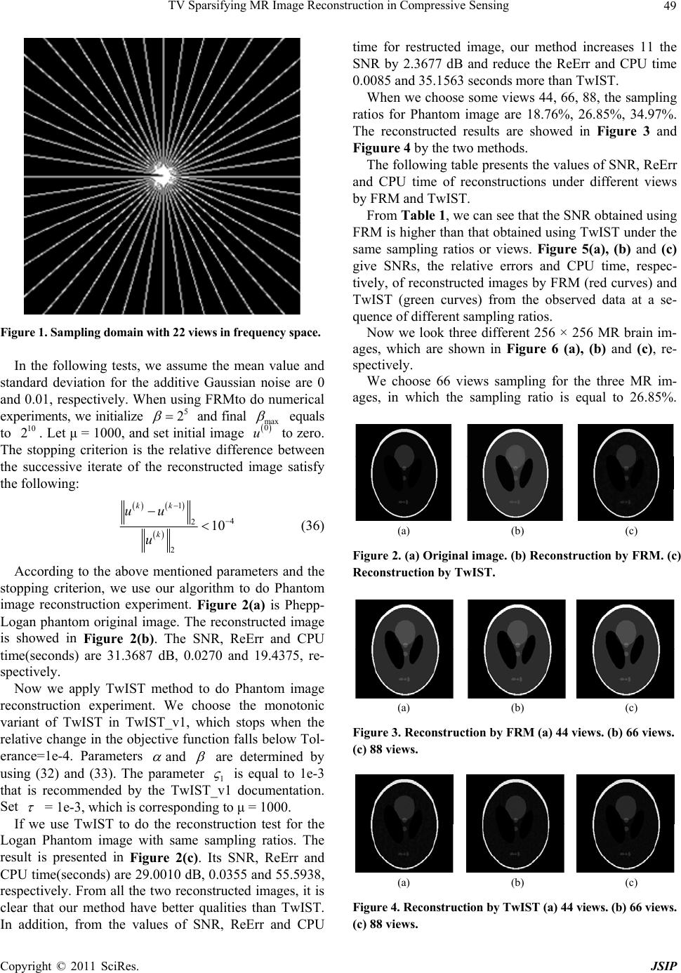

TV Sparsifying MR Image Reconstruction in Compressive Sensing 49
Figure 1. Sampling domain with 22 views in frequen cy sp ace.
In the following tests, we assume the mean value and
standard deviation for the additive Gaussian noise are 0
and 0.01, respectively. When using FRMto do numerical
experiments, we initialize 5 2   and final max

equals
to 10 2. Let μ = 1000, and set initial image

0
u to zero.
The stopping criterion is the relative difference between
the successive iterate of the reconstructed image satisfy
the following:
 

1
4
2
2
10
kk
k
uu
u


 (36)
According to the above mentioned parameters and the
stopping criterion, we use our algorithm to do Phantom
image reconstruction experiment. Figure 2(a) is Phepp-
Logan phantom original image. The reconstructed image
is showed in Figure 2(b). The SNR, ReErr and CPU
time(seconds) are 31.3687 dB, 0.0270 and 19.4375, re-
spectively.
Now we apply TwIST method to do Phantom image
reconstruction experiment. We choose the monotonic
variant of TwIST in TwIST_v1, which stops when the
relative change in the objective function falls below Tol-
erance=1e-4. Parameters

and

are determined by
using (32) and (33). The parameter 1

is equal to 1e-3
that is recommended by the TwIST_v1 documentation.
Set

= 1e-3, which is corresponding to μ = 1000.
If we use TwIST to do the reconstruction test for the
Logan Phantom image with same sampling ratios. The
result is presented in Figure 2(c). Its SNR, ReErr and
CPU time(seconds) are 29.0010 dB, 0.0355 and 55.5938,
respectively. From all the two reconstructed images, it is
clear that our method have better qualities than TwIST.
In addition, from the values of SNR, ReErr and CPU
time for restructed image, our method increases 11 the
SNR by 2.3677 dB and reduce the ReErr and CPU time
0.0085 and 35.1563 seconds more than TwIST.
When we choose some views 44 , 66, 88, the sampling
ratios for Phantom image are 18.76%, 26.85%, 34.97%.
The reconstructed results are showed in Figure 3 and
Figuure 4 by the two methods.
The following table presents the values of SNR, ReErr
and CPU time of reconstructions under different views
by FRM and TwIST.
From Table 1, we can see that the SNR obtain ed using
FRM is higher than that obtained using TwIST under the
same sampling ratios or views. Figure 5(a), (b) and (c)
give SNRs, the relative errors and CPU time, respec-
tively, of reconstructed images by FRM (red curves) and
TwIST (green curves) from the observed data at a se-
quence of different sampling ratios.
Now we look three different 256 × 256 MR brain im-
ages, which are shown in Figure 6 (a), (b) and (c), re-
spectively.
We choose 66 views sampling for the three MR im-
ages, in which the sampling ratio is equal to 26.85%.
(a) (b) (c)
Figure 2. (a) Original image. (b) Reconstruction by FRM. (c)
Reconstruction by TwIST.
(a) (b) (c)
Figure 3. Reconstruction by FRM (a) 44 views. (b) 66 views.
(c) 88 views.
(a) (b) (c)
Figure 4. Reconstruction by TwIST (a) 44 views. (b) 66 views.
(c) 88 views.

TV Sparsifying MR Image Reconstruction in Compressive Sensing 50
Table 1. SNR, ReErr, CPU of reconstructions under differ-
ent views or sampling ratios by two methods.
Views/Samp.ratio Method SNR ReErr CPU
FRM 40.6877 0.0092 7.1875
44/18.76% TwIST 30.7696 0.0289 26.4219
FRM 44.8714 0.0057 4.9063
66/26.85% TwIST 30.8412 0.0287 20.2031
FRM 47.8810 0.0040 3.6719
88/34.97% TwIST 30.8412 0.0286 17.7969
(a)
(b)
(c)
Figure 5. (a) SNRs. (b) Relative Errors. (c) CPU time.
When use FRM and TwIST to do reconstruction ex-
periments for the three MR images, all parameters in the
two methods are still same as the above mentioned. The
results reconstructed by FRM and TwIST are presented
in Figure 7. and Figure 8., respectively.
The SNRs, the relative errors and CPU time of the re-
constructed images by FRM and TwIST are given in the
Table 2.
From the quality of reconstructed images and the val-
ues of SNR, ReErr and CPU time, we can see that FRM
method is better than TwIST method.
(a) (b) (c)
Figure 6. Original image. (a) Brain 1. (b) Brain 2. (c) Brain 3.
(a) (b) (c)
Figure 7. Reconstructions by FRM (a) Brain 1. (b) Brain 2.
(c) Brain 3.
(a) (b) (c)
Figure 8. Reconstructions by TwIST (a) Brain 1. ( b) Br ain 2.
(c) Brain 3.
Table 2. SNR, ReErr, CPU time and sampling ratios for
reconstructed results by FMR and TwIST.
ImageMethodSNR ReErr CPU Samp.ratio
FRM 26.12880.0494 6.9063 26.85%
Brain
1 TwIST 24.73650.0580 20.8438 26.85%
FRM 21.93530.0800 9.1719 26.85%
Brain
2 TwIST 21.14940.0876 20.9375 26.85%
FRM 27.69160.0412 6.4531 26.85%
Brain
3 TwIST 26.15990.0492 20.5938 26.85%

TV Sparsifying MR Image Reconstruction in Compressive Sensing 51
5. Conclusion
We have developed a fast reconstruction method for
compressed sensing MRI that is called FRM. The con-
vergence of the reconstruction method has been analyzed.
The algorithm has been accelerated by continuation on
penalty parameters. FRM is compared with TwIST, a
state-of-the-art method. We use the two methods to re-
construct Phantom image and some real MR images from
a partial of observed data. The results of numerical ex-
periments on the MR images demonstrate that FRM can
achieve much higher performance in terms of SNRs, the
relative errors and CPU time than TwIST. We believe
that our method can be applied in the area of rapid MR
imaging.
6. Acknowledgements
This work was supported by the Key Project of Chinese
Ministry of Education(No. 109030), 382 Training Pro-
gramme of CUC(G08382316) and Science Research Pro-
ject of CUC(XNL1003). The authors would like to thank
the referees for very useful suggestions here.
REFERENCES
[1] E. J. Candes, J. Romberg, and T. Tao, “Robust uncer-
tainty principles: Exact signal reconstruction from highly
incomplete frequency information,” IEEE Trans. Inf. The-
ory, Vol. 52, 2006, pp. 489-509.
[2] D. L. Donoho, “Compressed sensing,” IEEE Trans. Inf.
Theory, Vol. 52, 2006, pp. 1289-1306.
[3] E. Candes and J. Romberg, “Sparsity and incoherence in
compressive sampling,” Inverse Problems, Vol. 23, 2007,
pp. 969-985.
[4] B. K. Natarajan, “Sparse approximate solutions to linear
systems,” SIAM J. Comput., Vol. 24, 1995, pp.227-234.
[5] D. Donoho and X. Huo, “Uncertainty principles and ideal
atomic decompositions,” IEEE Trans. Inf.Theory, Vol. 47,
2001, pp. 2845-2862.
[6] J. J. Fuchs, “On sparse representations in arbitrary redun-
dant bases,” IEEE Trans. Inf. Theory, Vol. 50, 2004, pp.
1341-1344.
[7] L. Rudin, S. Osher and E. Fatemi, “Nonlinear total varia-
tion based noise removal algorithms,” Physica D, Vol. 60,
1992, pp. 259-268.
[8] L. He, T. C. Chang, S. Osher, T. Fang and P. Speier, “MR
image reconstruction by using the iterative refinement
method and nonlinear inverse scale space methods,”
UCLA CAM Report, 2006,06-35.
[9] M. Lustig, D. Donoho and J. Pauly, “Sparse MRI: The
application of compressed sensing for rapid MR imag-
ing,” Magnetic Resonance in Medicine, Vol. 58,2007,pp.
1182-1195.
[10] Y. Wang, J. Yang, W. Yin and Y. Zhang, “A alternating
minimization algorithm for total variation image recon-
struction,” SIAM J. Imag. Sci., Vol. 1, 2008,pp. 248-272.
[11] R. Courant, “Variational methods for the solution of
problems with equilibrium and vibration,” Bull.Amer.
Math. Soc., Vol. 49, 1943, pp. 1-23.
[12] M. K. Ng, R. H. Chan and W. C. Tang, “A fast algorithm
for deblurring models with Neumann boundary condi-
tions,” SIAM J. Sci. Comput., Vol. 21, pp. 851-866, 1999.
[13] Z. Opal, “Weak convergence of the sequence of succes-
sive approximations for nonexpansive mappings,” Bull.
Amer. Math. Soc., Vol. 73, 1967, pp. 591-597.
[14] J. Yang, W. Yin and Y.Wang, “A Fast Algorithm for
Edge-Preserving Variational Multichannel Image Resto-
ration,” SIAM J. Sci. Comput., Vol. 2, 2009, pp. 569-592.
[15] J. Yang, Y. Zhang and W. Yin, “A Fast Alternating Di-
rection Method for TVL1-L2 Signal Reconstruction From
Partial Fourier Data,” IEEE Journal of Selected Topics in
Signal Processing, Vol. 4, 2010, pp.288-297.
[16] E. T. Hale, W. Yin and Y. Zhang, “A Fixed-Point Con-
tinuation for l1−regularization with Application to Com-
pressed Sensing,” Rice University CAAM Technical Re-
port TR07-07, 2007, pp. 1-45.
[17] E. T. Hale, W. Yin and Y. Zhang, “Fixed-Point Continua-
tion for l1−Minimization: Methodology and Conver-
gence,” SIAM J. Sci. Comput., Vol. 2, 2009, pp. 569-592.
[18] J. Bioucas-Dias and M. Figueiredo, “A new TwIST:
Two-step iterative thresholding algorithm for image res-
toration,” IEEE Trans. Imag. Process., Vol. 16, 2007, pp.
2992-3004.
[19] I. Daubechies, M. Defriese and C. De Mol, “An iterative
thresholding algorithm for linear inverse problems with a
sparsity constraint,” Commun. Pure Appl. Math., Vol. 57,
2004, pp. 1413-1457.
[20] A. Chambolle, “An algorithm for total variation minimi-
zation and applications,” J. Math. Imaging Vision, Vol.
20, 2004, pp. 89-97.