J
ournal o
f
A
pp
http://dx.doi.or
g
Copyright © 2
0
An E
P
und
e
ABSTRA
C
In this paper,
credit periods
money from
m
p
eriod to his
r
tory model h
a
non-linear op
t
Lastly Numer
Keywords: E
1. Introdu
c
N
ormally, th
e
tailer to the s
u
the consignm
e
in the market
offered by th
e
the trade cre
d
accumulate r
e
p
lored a singl
in payments
a
optimal solut
i
However, the
in the above
Goyal’s mod
e
et al. [4] furt
h
to allow for s
h
el to determi
n
ing items un
d
and allowabl
e
model for de
t
supplier offer
s
order quantit
y
Chung and H
u
the case that
t
der delay in
p
credit financi
either consta
n
Liao et al. [8]
p
lied Mathemat
i
g
/10.4236/jamp
.
0
13 SciRes.
P
Q-Ba
s
e
r Stoc
k
Departmen
t
C
T
an EPQ-
b
ase
d
. In addition,
t
m
oney lendin
g
r
etailer and re
t
a
s been formu
l
t
imization me
ical examples
PQ Model; I
m
c
tion
e
payment for
u
pplier imme
d
e
nt. Nowaday
s
to attract mor
e
e
supplier to t
h
d
it period, th
e
e
venue and ea
r
e item EOQ
m
a
nd Chung [2
]
i
on for the
p
r
o
phenomenon
models. Agg
a
e
l to the case
w
h
er generaliz
e
h
ortages. Sark
n
e an optimal
o
d
er inflation,
p
e
shortage. C
h
t
eriorating ite
m
s
a permissibl
e
y
is greater t
h
u
ang [7] furth
e
t
he units are r
p
ayments. All
ng assumed
t
n
t or merely d
e
considered a
n
i
cs and Ph
y
sics
,
.2013.14005 P
u
s
ed Inv
k
-Depe
t
of Mathemati
c
p
in
k
d
inventory p
o
t
here is a pro
v
g
source for th
t
ailer also off
e
l
ated with res
p
tho
d
-Generali
z
are set to illu
s
m
mediate Part
P
an order is
m
d
iately just aft
e
s
, due to the
s
e
customers,
a
h
e retailer. B
e
e
retailer can
r
n interest. G
o
m
odel under p
e
]
simplified t
h
o
blem explore
of deteriorati
a
rwal and Jag
w
ith deteriorat
i
e
d the above i
n
er et al. [5] d
e
o
rdering polic
y
p
ermissible de
l
h
ang [6] esta
b
m
s under inf
l
e
delay to the
h
an a predeter
m
e
r extended
G
eplenished at
the above pa
p
t
hat the mark
e
e
pendent on t
h
n
initial-stock-
l
,
2013, 1, 25-3
0
u
blished Online
O
entory
ndent
D
P
a
P. Maju
m
c
s, National Inst
i
k
ff
Rece
o
licy for an it
e
v
ision for 1) a
n
e immediate
p
e
rs a trade cre
d
p
ect to the ret
a
z
ed Reduced
s
trate this mod
P
aymen
t
m
ade by the
r
e
r the receipt
o
s
tiff competiti
o
a
credit period
e
fore the en
d
o
sell the goo
d
o
yal [1] first e
x
e
rmissible del
a
h
e search of t
h
d
by Goyal [
1
on was ignor
e
g
i [3] extend
e
i
ng items. Ja
m
n
ventory mo
d
e
veloped a mo
d
y
for deterior
a
l
ay in payme
n
b
lished an EO
l
ation when t
h
purchaser if t
h
m
ined quantit
y
G
oyal’s model
t
a finite rate u
n
p
ers under tra
d
e
t demand w
a
h
e retailing pri
c
l
evel-depende
n
0
O
ctobe
r
2013 (
h
Model
D
eman
d
a
yment
m
der, U. K.
B
i
tute of Techno
l
ff
mail.com, ber
a
ive
d
July 2013
e
m is present
e
n
immediate p
p
art paymen
t
,
3
d
it period to
h
a
iler’s point o
f
Gradient (G
R
el. Finally we
e-
o
f
o
n
is
o
f
d
s,
x
-
a
y
h
e
1
].
e
d
e
d
m
al
d
el
d
-
a
t-
n
ts
Q
h
e
h
e
y
.
t
o
n
-
d
e
a
s
c
e
nt
deman
d
retailer
Chaud
h
rent-st
o
gives
a
on the
velope
d
deman
d
p
rogre
s
stock-
d
menon
.
a com
m
above
m
retailer
trade c
r
transac
t
is unre
adopt t
h
mote
m
repleni
s
and Z
h
stock-
d
period.
N
o
w
wholes
eral m
e
terms
o
retailer
h
ttp://www.scir
p
for De
t
d
with
I
B
era
l
ogy, Agartala,
B
a
e
d with stoc
k
-
d
art payment t
o
3
) here suppli
e
h
is customer.
A
f
view for min
i
R
G) method is
use LINGO s
o
d
rate, i.e. th
e
’s order qu
a
h
uri [9] analy
z
o
c
k
-dependent
a
retailer both
purchase of
m
d
the optimal
d
is stoc
k
-dep
e
s
sive credit pe
r
d
ependent fail
e
.
In the real li
f
m
on phenom
e
m
odel assum
e
a delay perio
d
r
edit period to
t
ions, especia
l
alistic. Huan
g
h
e trade credi
t
m
arket comp
e
s
hment model
h
ao [11] int
r
d
ependent de
m
w
adays for th
e
aler tries to
m
e
ans. For thi
s
o
f unit price,
c
s against im
m
p
.org/journal/ ja
m
t
eriora
t
I
mmed
i
B
arjala, Jirania,
.co.in
d
ependent de
m
o
the wholesal
e
r or wholesal
A
gainst the ab
o
i
mizing the to
t
used to find
o
ftware to sol
v
e
demand rat
e
a
ntity. More
z
ed a kind of
demand rat
e
a credit perio
d
m
erchandise. S
ordering po
l
e
ndent and w
h
r
iods. But the
s
e
d to conside
r
f
e, however, d
e
e
non. On the
o
e
d that the su
p
d
but the retai
l
his/her custo
m
l
ly in supply
c
g
assumed tha
t
t
policy to his
e
tition and de
tha
t
is a two-
r
oduce
d
an i
n
m
and under t
w
e
speedy m
o
m
aximize his/h
e
s
, very often
c
redit period
e
m
ediate part p
a
m
p )
t
ing Ite
m
i
ate Pa
r
India
m
and during t
w
e
r
, 2) borrow
i
er offers a tra
d
o
ve conjectur
e
t
al inventory
c
the optimal s
o
v
e this model.
e
is influence
d
recently, S
a
EOQ model
w
e
where the
d
and a price
oni and Shah
l
icy for retail
h
en supplier o
f
s
e models wit
h
r
deterioratio
n
e
terioration o
f
o
ther hand, t
h
p
plier would
o
l
er would not
m
ers. In most
c
hain, this as
s
t
the retailer
w
/her customer
veloped the
r
level trade cr
e
n
ventory mo
d
w
o level of tra
d
o
vement of c
a
e
r market thro
u
some conce
s
e
tc. are offer
e
a
yment. To a
v
JAMP
m
s
r
t
w
o trade
i
ng some
d
e credit
e
s inven-
c
ost. The
o
lutions.
d
by the
a
na and
w
ith cur-
supplier
discount
[10] de-
er when
f
fers two
h
current
n
pheno-
f
items is
h
e entire
o
ffer the
offer the
business
s
umption
w
ill also
s to p
r
o-
r
etailer’s
e
dit. Min
d
el with
d
e credit
a
pital, a
u
gh sev-
s
sions in
e
d to the
v
ail these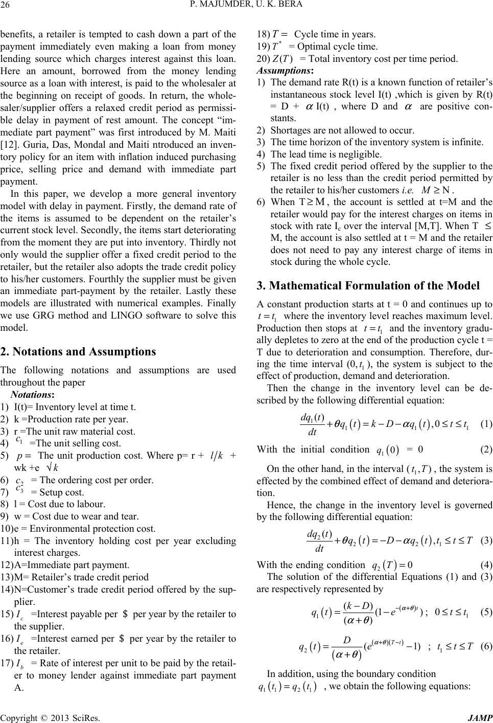

P. MAJUMDER, U. K. BERA
26
benefits, a retailer is tempted to cash down a part of the
payment immediately even making a loan from money
lending source which charges interest against this loan.
Here an amount, borrowed from the money lending
source as a loan with interest, is paid to the wholesaler at
the beginning on receipt of goods. In return, the whole-
saler/supplier offers a relaxed credit period as permissi-
ble delay in payment of rest amount. The concept “im-
mediate part payment” was first introduced by M. Maiti
[12]. Guria, Das, Mondal and Maiti ntroduced an inven-
tory policy for an item with inflation induced purchasing
price, selling price and demand with immediate part
payment.
In this paper, we develop a more general inventory
model with delay in payment. Firstly, the demand rate of
the items is assumed to be dependent on the retailer’s
current stock level. Secondly, the items start deteriorating
from the moment they are put into inventory. Thirdly not
only would the supplier offer a fixed credit period to the
retailer, but the retailer also adopts the trade credit policy
to his/her customers. Fourthly the supplier must be given
an immediate part-payment by the retailer. Lastly these
models are illustrated with numerical examples. Finally
we use GRG method and LINGO software to solve this
model.
2. Notations and Assumptions
The following notations and assumptions are used
throughout the paper
Notations:
1) I(t)= Inventory level at time t.
2) k =Production rate per year.
3) r =The unit raw material cost.
4) 1
c =The unit selling cost.
5) p= The unit production cost. Where p= r + lk +
wk +e k√
6) 2 c = The ordering cost per order.
7) 3
c = Setup cost.
8) l = Cost due to labour.
9) w = Cost due to wear and tear.
10) e = Environmental protection cost.
11) h = The inventory holding cost per year excluding
interest charges.
12) A=Immediate part payment.
13) M= Retailer’s trade credit period
14) N=Customer’s trade credit period offered by the sup-
plier.
15) c
I
=Interest payable per $ per year by the retailer to
the supplier.
16) e
I
=Interest earned per $ per year by the retailer to
the retailer.
17) b
I
= Rate of interest per unit to be paid by the retail-
er to money lender against immediate part payment
A.
18) T= Cycle time in years.
19) * T = Optimal cycle time.
20) ()
Z
T = Total inventory cost per time period.
Assumptions:
1) The demand rate R(t) is a known function of retailer’s
instantaneous stock level I(t) ,which is given by R(t)
= D +
α I(t) , where D and α are positive con-
stants.
2) Shortages are not allowed to occur.
3) The time horizon of the inventory system is infinite.
4) The lead time is negligible.
5) The fixed credit period offered by the supplier to the
retailer is no less than the credit period permitted by
the retailer to his/her customers i.e. NM≥.
6) When TM≥, the account is settled at t=M and the
retailer would pay for the interest charges on items in
stock with rate Ic over the interval [M,T]. When T ≤
M, the account is also settled at t = M and the retailer
does not need to pay any interest charge of items in
stock during the whole cycle.
3. Mathematical Formulation of the Model
A constant production starts at t = 0 and continues up to
1
tt= where the inventory level reaches maximum level.
Production then stops at 1 tt= and the inventory gradu-
ally depletes to zero at the end of the production cycle t =
T due to deterioration and consumption. Therefore, dur-
ing the time interval (0, 1
t), the system is subject to the
effect of production, demand and deterioration.
Then the change in the inventory level can be de-
scribed by the following differential equation:
() ()
1
111
() ,0 dq tqtk Dqttt
dt
θα +=−− ≤≤ (1)
With the initial condition
()
10q = 0 (2)
On the other hand, in the interval (1,)tT, the system is
effected by the combined effect of demand and deteriora-
tion.
Hence, the change in the inventory level is governed
by the following differential equation:
() ()
2
221
() , dq tqtDqtt tT
dt
θα +=−− ≤≤ (3)
With the ending condition
()
20qT= (4)
The solution of the differential Equations (1) and (3)
are respectively represented by
()
()
1
()
(1 )
()
t
kD
qt e
αθ
αθ
−+
−
=−
+; 1
0tt≤≤ (5)
() ()
()()
2(1)
Tt
D
qt e
αθ
αθ
+−
=−
+ ; 1
ttT≤≤ (6)
In addition, using the boundary condition
() ()
11 21
qt qt= , we obtain the following equations: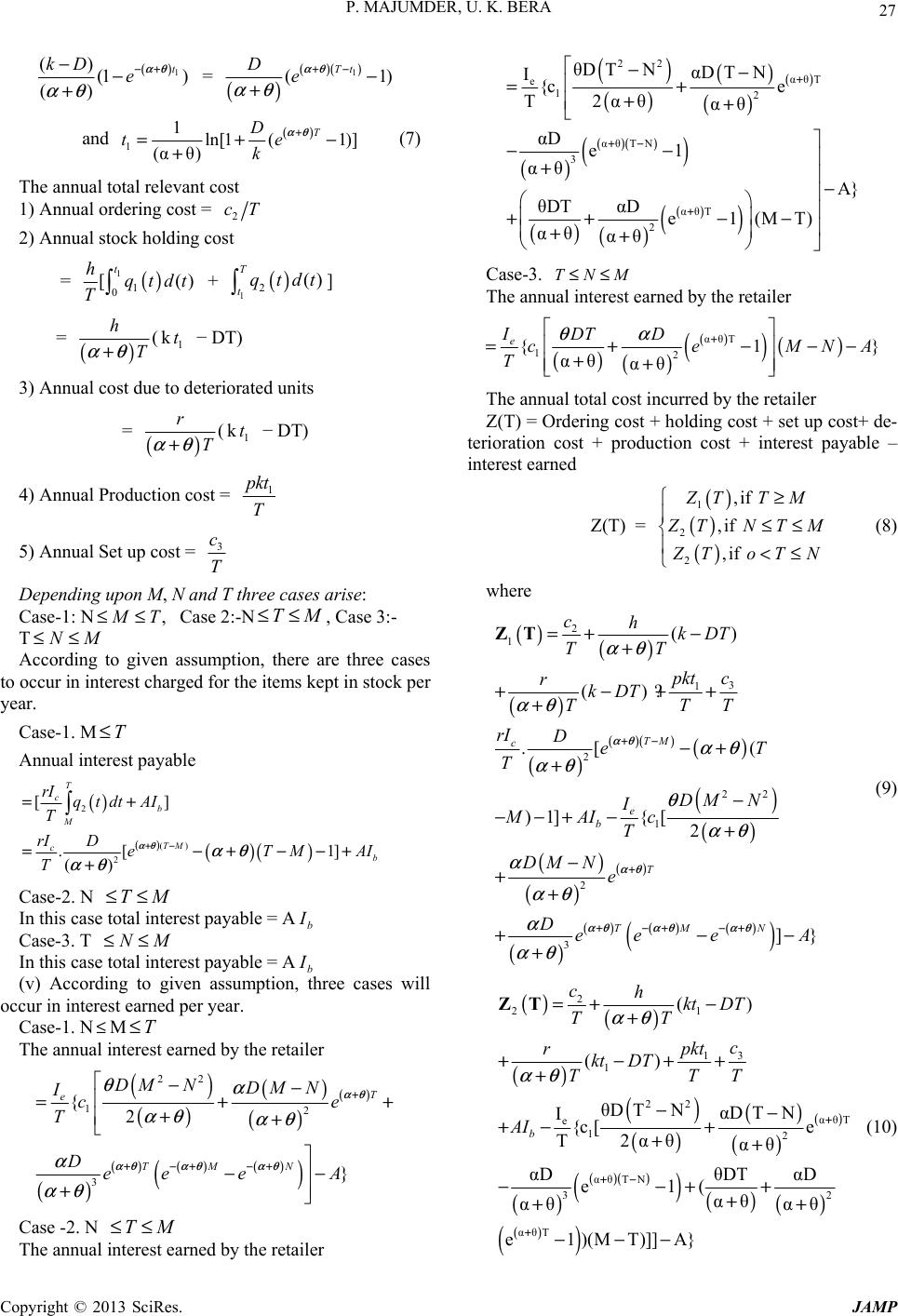

P. MAJUMDER, U. K. BERA
27
()
1
()
(1 )
()
t
kD e
αθ
αθ
−+
−−
+ =
()
()()
1
(1)
Tt
De
αθ
αθ
+−
−
+
and
()
1
1ln[1 (1)]
(αθ)
T
D
te
k
αθ +
=+−
+ (7)
The annual total relevant cost
1) Annual ordering cost = 2
cT
2) Annual stock holding cost
=
()
1
1
0
[()
t
hqtdt
T +
()
12()
T
tqtdt
]
=
()
(
h
T
αθ +k1
t − DT)
3) Annual cost due to deteriorated units
=
()
(
r
T αθ +k1
t − DT)
4) Annual Production cost = 1
pkt
T
5) Annual Set up cost = 3
c
T
Depending upon M , N and T three cases arise:
Case-1: N,
M
T≤≤ Case 2:-NTM≤≤ , Case 3:-
TNM≤≤
According to given assumption, there are three cases
to occur in interest charged for the items kept in stock per
year.
Case-1. MT≤
Annual interest payable
()
()
()( )
2
()
2
]
.[ 1]
()
[
T
cb
M
TM
cb
rI qtdt AI
T
rID eTMAI
T
αθ
αθ
αθ
+−
=+
=−+−−+
+

Case-2. N TM≤≤
In this case total interest payable = Ab
I
Case-3. T NM≤≤
In this case total interest payable = Ab
I
(v) According to given assumption, three cases will
occur in interest earned per year.
Case-1. N≤MT≤
The annual interest earned by the retailer
()
()
()
()
()
()
() ()()
()
22
12
3
{2
}
T
e
TM N
DM NDM N
Ice
T
Dee eA
αθ
αθ αθαθ
θα
αθ αθ
α
αθ
+
+−+−+
−−

=++
+ +


−− 
+

Case -2. N TM≤≤
The annual interest earned by the retailer
()
()
()
()
()
()
()( )
()
()
()
()
()
22
αθT
e
12
αθ TN
3
αθT
2
θDTNαDT N
I{c e
T2αθ αθ
αDe1
αθ
A}
θDT αDe1(MT)
αθ αθ
+
+−
+
−−
=+
++
−−
+−

 +







+−−

+




+

Case-3. TNM≤≤
The annual interest earned by the retailer
()
()
()
()
()
αθT
12
{1}
αθ αθ
e
IDT D
ceMNA
T
θα
+

=+ −−− 
++


The annual total cost incurred by the retailer
Z(T) = Ordering cost + holding cost + set up cost+ de-
terioration cost + production cost + interest payable –
interest earned
Z(T) =
()
()
()
1
2
2
,if
,if
,if
ZTTM
Z
TNTM
Z
ToTN
≥ 
≤≤

<≤

(8)
where
() ()
()
()
()( )
()
()
()
()
()
()
()
() ()()
()
2
1
3 1
2
22
1
2
3
(
( ?
.[ (
)1][ 2
)
]
)
{
}
TM
c
e
b
T
TM N
chkDT
TT
c
pkt rkDT
TTT
rI DeT
T
DM N
I
MAIc
T
DM Ne
Dee eA
αθ
αθ
αθ αθαθ
αθ
αθ
αθ
αθ
θ
αθ
α
αθ
α
αθ
+−
+
+−+−+
=+ −
+
+−++
+
−+
+
−
−−+ −+
−
++
+−−
+
ZT
(9)
() ()
()
()
()
()
()
()
()
()( )
()
()
()
()
()
2
21
3 1
1
22
αθT
e
12
αθ TN
32
αθT
(
(
θDT NαDT N
I{c e
T2αθ αθ
αDθDT αD
e1(
αθ
αθ αθ
e1 )(MT)]]
)
}
)
A
[
b
chkt DT
TT
c pkt
rkt DT
TTT
AI
αθ
αθ
+
+−
+
=+ −
+
+−++
+
−−
+− +
++
−−++
+
++
−−−
ZT
(10)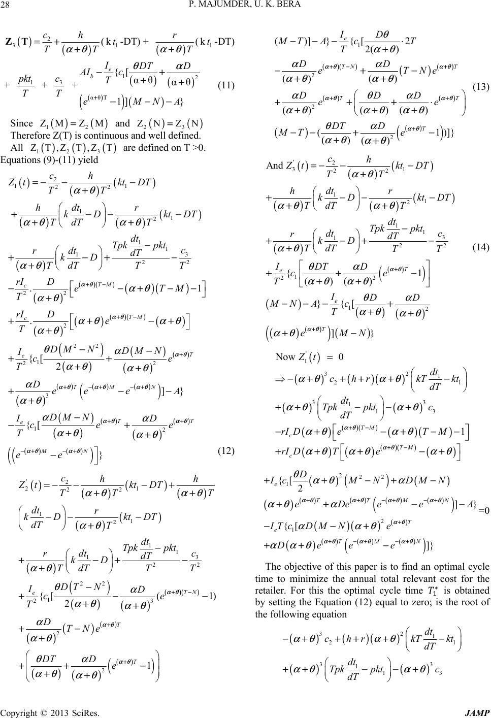

P. MAJUMDER, U. K. BERA
28
() ()
2
3(
ch
TT
αθ
=++ ZT k1
t-DT) +
()
(
r
T
αθ +k1
t-DT)
+ 1
pkt
T + 3
c
T +
()
()
()
()
()
12
αθT
[{αθ αθ
1] }
e
b
IDT D
AI c
T
eMNA
θα
+
−+
++
−−−
(11)
Since
() ()
12
ZMZ M= and
() ()
23
ZN ZN=
Therefore Z(T) is continuous and well defined.
All
() () ()
123
ZT,Z T,ZT
are defined on T >0.
Equations (9)-(11) yield
() () ()
() ()
()
()
()
()( )
()()
()
()
()()
()
()
()
()
()
()
()
'2
11
22
1
1
2
1
13
1
22
22
2
22
1
22
3
.
[
1
.
{2
TM
c
TM
c
T
e
ch
Ztkt DT
TT
dt hr
kD ktDT
TdT T
dt
Tpkpkt c
dt rdT
kD
TdT TT
rI DeTM
T
rI De
T
DM NDM N
Ice
T
D
αθ
αθ
αθ
αθ
αθ αθ
αθ
αθ
αθ
αθ αθ
αθ
θα
αθ αθ
α
αθ
+−
+−
+
=− −−
+

+−−−

++

−

+−+−

+

−−+−−

+

++−+

+
−−
++
++
++
() ()()
()
()
()
()
()
()
() ()
()
(
12
]}
{[
}
TM N
TT
e
MN
ee eA
DMN
ID
ce e
T
ee
αθ αθαθ
αθ αθ
αθ αθ
αα
αθ αθ
+−+ −+
++
−+ −+
−−
−
−+
++

− (12)
() () ()
()
()
()
()
()
()
()
()()
()
()
()
()
()
()
()
'2
21
22
1
1
2
1
13
1
22
22
1
23
2
2
{(1)
2
1
[TN
e
T
T
chh
ZtktDTT
TT
dt r
kD ktDT
dT T
dt
Tpkpkt c
dt rdT
kD
TdT TT
DT N
ID
ce
T
DTNe
DTD e
αθ
αθ
αθ
αθ
αθ
αθ
αθ
θα
αθ αθ
α
αθ
θα
αθ αθ
+−
+
+
=−−−++
+

−− −

+

−

+−+−

+
−
+−−
++
+−
+

 ++ −

++

()( )
()
()
() ()
()
()
()
1
2
2
2
()]}{[2
2( )
()
()
()() ()
(1 )]}
() ()
e
TN T
TT
T
ID
MT AcT
T
DD
eTNe
DDD
ee
DT D
MT e
αθ αθ
αθ αθ
αθ
θ
αθ
αα
αθ αθ
αθα
αθ αθ αθ
θα
αθ αθ
+− +
++
+
−−− ⋅
+
−+−
+
+

+++⋅

++ +
−− +−
++
(13)
() () ()
() ()
()
()
()
()
() ()
()
()
()
()
()
'2
31
22
1
1
2
1
13
1
22
1
22
12
And
{1
() ()
}{
]}
[
T
e
e
T
ch
Ztkt DT
TT
dt hr
kD ktDT
TdT T
dt
Tpkpkt c
dt rdT
kD
TdT TT
IDT D
ce
T
IDD
MN Ac
T
eMN
αθ
αθ
αθ
αθ αθ
αθ
θα
αθ αθ
θα
αθ αθ
αθ
+
+
−− −
+

+−−−

++

−

+−+−

+

++ −

++

−−− +
++
+−
=
(14)
()
()()()
() ()
()
()( )
()()
()()
()()
()
'
1
32
1
21
33
1
13
Now 0
1
TM
c
TM
c
Zt
dt
chrkT kt
dT
dt
Tpk pktc
dT
rI DeTM
rI DTe
αθ
αθ
αθ αθ
αθ αθ
αθ αθ
αθ αθαθ
+−
+−
=

−+++ +−



++− −+




−+ −+−−




++ +−+


()
()
()
()
()() ()()
()
()()
()
()
() ()()
()
222
1
2
1
2
{[
]}
{
}
[
]
e
TTMN
T
e
TM N
D
IcMNDM N
eDeee A
IT cDMNe
Dee e
αθαθαθαθ
αθ
αθ αθαθ
θαθ α
αθ α
ααθ
ααθ
++ −+−+
+
+−+−+
++−+−
++ −−
−−+
++ −
=0
The objective of this paper is to find an optimal cycle
time to minimize the annual total relevant cost for the
retailer. For this the optimal cycle time 

∗ is obtained
by setting the Equation (12) equal to zero; is the root of
the following equation
()()()
() ()
32
1
21
33
1
13
dt
chrkT kt
dT
dt
Tpk pktc
dT
αθαθ
αθ αθ

−+++ +−



++−−+



P. MAJUMDER, U. K. BERA
29
()
()( )
()()
()()
()()
()
1
TM
c
TM
c
rI DeTM
rI DTe
αθ
αθ
αθ αθ
αθ αθαθ
+−
+−

−+ −+−−


++ +−+

()
()
()
()
()() ()()
()
()()
()
()
() ()()
()
222
1
2
1
2
{[
]}
{
0
[
]
e
TTMN
T
e
TM N
D
IcMNDM N
eDeee A
IT cDMNe
Dee e
αθαθ αθαθ
αθ
αθ αθαθ
θαθ α
αθ α
ααθ
ααθ
++ −+−+
+
+−+ −+
++−+−
++ −−
−−+
++ −
=
(15)
()
Equation15is the optimality condition of (9)
Now '
2
Z
(t) = 0
()()()
() ()
()
()
()
()
()()( )
()
() ()
()
() ()
() ()
()( )
()()
()
()
()
()
32
1
21
33
1
13
222
1
2
2
1
2
2
{[
2
1
1( )]
}{[
e
TTN
T
TN
e
TT
dt
chrkT kt
dT
dt
Tpkpktc
dT
D
IcTNDT N
eDe
DTDeM T
AITcDT De
DTNeDe
D
αθ αθ
αθ
αθ
αθ αθ
αθ αθ
αθ αθ
θαθα
αθ α
θαθααθ
θα θααθ
ααθ ααθ
θαθ
++−
+
+−
++

−+++ +−



++− −+


++−+−
+− −
++++ −−
−−+ −+
++−+ +
++
()
()
()
()
() ()
()
()
()
2
21]}
0
T
T
DeMT
DT De
αθ
αθ
ααθ
αθθααθ
+
+
++−
−++ +−
=
(16)
()
Equation16is the optimality conditionof (10)
Again '
3
Z
(t) = 0
()()()
() ()
() ()
()
()
()
() ()
()
()
32
1
21
33
1
13
2
1
22
1
1{[ ]
}
{
}0
T
e
T
e
dt
chrkT kt
dT
dt
Tpk pktc
dT
IcDT De
MN A
IT cDDe
MN
αθ
αθ
αθ αθ
αθ αθ
θα θααθ
θαθ ααθ
+
+

−+++ +−



++− −+


++++ −
−−

−+++

−=
(17)
()
Equation17is the optimality conditionof (11)
4. Numerical Examples
To illustrate the results of the proposed model we solve
the following numerical examples
Example 1. When1150 /,c Rsunit=
2100 /cRsorder=, 350cRs=, M = 0.5 year, N = 0.01
year, D = 1500 units per year , k = 2000 units/year, A =
Rs 700 , h = Rs 15/unit,
r = Rs 4/unit, l = Rs200, w = Rs 0.0005, e = Rs 0.1,
0.12
e
I=, 0.17
c
I=, 0.15
b
I=, 0.2,0.2 αθ ==
then the optimal value of T is *
15.231635T=and
*
11
Z ()30310.78T=
Example 2. When1150 /,c Rsunit=
2100 /cRsorder=, 350cRs=, M = 2.5 year, N = 0.01
year, D = 1000 units per year , k = 2500 units/year, A =
Rs 2000 , h = Rs 10/unit,
r = Rs 4/unit, l = Rs200, w = Rs 0.05, e = Rs 0.1,
0.12
e
I=, 0.17
c
I=, 0.15
b
I=, 0.1,0.1 αθ == then
the optimal value of T is *
21.068099T= and
*
22
Z ()165639.8T=
Example 3. When
1136 /,c Rsunit=2100 /cRs order=,330cRs=, M=2.1
year, N =1.07 year, D = 2000 units per year , k = 2500
units/year, A = Rs 2800 , h = Rs 10/unit, r = Rs 4/unit, l
= Rs100 , w = Rs 0.05, e = Rs 0.1, 0.15
e
I=,
0.20
c
I=, 0.12
b
I= , 0.1,0.1 αθ == then the op-
timal value of T is *
30.9165449T=and
*
33
Z ()79741.83T=
5. Conclusions
In this paper, we develop an EPQ model for deteriorating
items under permissible delay in payments. The primary
difference of this paper as compared to previous studies
is that we introduced a generalized inventory model by
relaxing the traditional EOQ model in the following
seven ways: 1) the demand of the items is dependent on
the retailer’s current stock level, 2) the retailer’s selling
price per unit is higher than its purchase unit cost, 3)
many items deteriorate continuously such as fruits and
vegetables, 4) the supplier not only would offer a fixed
credit period to the retailer, but the retailer also adopts
the trade credit policy to promote market competition, 5)
supplier must be given an immediate part payment by the
retailer after receipt of goods, 6) minimizing inventory
cost is used as the objective to find the optimal reple-
nishment policy. Three numerical examples are set to
illustrate this model. For the first example, *
1
T is the
optimal value of T, for second and third, the optimal
value of T is *
2
T and *
3
T respectively. This presented
model can be further extended to some more practical
situations, such as we could allow for shortages. Also
quantity discounts, time value of money and inflation etc.
may be added in this paper.
REFERENCES
[1] S. K. Goyal, “Economic Order Quantity under Conditions
of Permissible Delay in Payments,” The Journal of the

P. MAJUMDER, U. K. BERA
30
Operational Research Society, Vol. 36, No. 4, 1985, pp.
335-338.
[2] K. J. Chung, “A Theorem on the Determination of Eco-
nomic Order Quantity under Conditions of Permissible
Delay in Payments,” Computers & Operations Research,
Vol. 25, No. 1, 1998, pp. 49-52.
[3] S. P. Aggarwal and C. K. Jaggi, “Ordering Policies of
Deteriorating Items under Permissible Delay in Payments,”
The Journal of the Operational Research Society, Vol. 46,
No. 5, 1995, pp. 658-662.
[4] A. M. M. Jamal, B. R. Sarker and S. Wang, “An Ordering
Policy for Deteriorating Items with Allowable Shortages
and Permissible Delay in Payment,” The Journal of the
Operational Research Society, Vol. 48, 1997, pp. 826-
833.
[5] B. R. Sarker, A. M. M. Jamal and S. Wang, “Supply
Chain Model for Perishable Products under Inflation and
Permissible Delay in Payment,” Computers & Operations
Research, Vol. 27, No. 1, 2000, pp. 59-75.
http://dx.doi.org/10.1016/S0305-0548(99)00008-8
[6] C. T. Chang, “An EOQ Model with Deteriorating Items
under Inflation When Supplier Credits Linked to Order
Quantity,” International Journal of Production Econom-
ics, Vol. 88, No. 3, 2004, pp. 307-316.
http://dx.doi.org/10.1016/S0925-5273(03)00192-0
[7] K. J. Chung and Y. F. Huang, “The Optimal Cycle Time
for EPQ Inventory Model under Permissible Delay in
Payments,” International Journal of Production Eco-
nomics, Vol. 84, No. 3, 2003, pp. 307-318.
http://dx.doi.org/10.1016/S0925-5273(02)00465-6
[8] H. C. Liao, C. H. Tsai and C. T. Su, “An Inventory Model
with Deteriorating Items under Inflation When a Delay in
Payment Is Permissible,” International Journal of Pro-
duction Economics, Vol. 63, No. 2, 2000, pp. 207-214.
http://dx.doi.org/10.1016/S0925-5273(99)00015-8
[9] S. S. Sana and K. S. Chaudhuri, “A Deterministic EOQ
Model with Delays in Payments and Price-Discount Of-
fers,” European Journal of Operational Research, Vol.
184, No. 2, 2008, pp. 509-533.
http://dx.doi.org/10.1016/j.ejor.2006.11.023
[10] H. Soni and N. H. Shah, “Optimal Ordering Policy for
Stock-Dependent Demand under Progressive Payment
Scheme,” European Journal of Operational Research,
Vol. 184, No. 1, 2008, pp. 91-100.
http://dx.doi.org/10.1016/j.ejor.2006.10.048
[11] J. Min, Y.-W. Zhou and J. Zhao, “An Inventory Model
for Deteriorating Items under Stock-Dependent Demand
and Two-Level Trade Credit,” Applied Mathematical
Modelling, Vol. 34, No. 11, 2010, pp. 3273-3285.
http://dx.doi.org/10.1016/j.apm.2010.02.019
[12] A. Guria, B. Das, S. Mondal and M. Maiti, “Inventory
Policy for an Item with Inflation Induced Purchasing
Price, Selling Price and Demand with Immediate Part
Payment,” Applied Mathematical Modelling, Vol. 37, No.
1-2, 2013, pp. 240-257.