Applied Mathematics
Vol.3 No.10A(2012), Article ID:24149,13 pages DOI:10.4236/am.2012.330215
Empirical Review of Standard Benchmark Functions Using Evolutionary Global Optimization
Institut für Physikalische Chemie, Christian-Albrechts-Universität Kiel, Kiel, Germany
Email: hartke@pctc.uni-kiel.de
Received July 17, 2012; revised August 17, 2012; accepted August 25, 2012
Keywords: Optimization; Genetic Algorithms; Benchmark Functions; Dimensionality Scaling; Crossover Operators
ABSTRACT
We have employed a recent implementation of genetic algorithms to study a range of standard benchmark functions for global optimization. It turns out that some of them are not very useful as challenging test functions, since they neither allow for a discrimination between different variants of genetic operators nor exhibit a dimensionality scaling resembling that of real-world problems, for example that of global structure optimization of atomic and molecular clusters. The latter properties seem to be simulated better by two other types of benchmark functions. One type is designed to be deceptive, exemplified here by Lunacek’s function. The other type offers additional advantages of markedly increased complexity and of broad tunability in search space characteristics. For the latter type, we use an implementation based on randomly distributed Gaussians. We advocate the use of the latter types of test functions for algorithm development and benchmarking.
1. Introduction
Global optimization has a lot of real-world applications, both of discrete and non-discrete nature. Among them are chemical applications such as structure optimization of molecules and clusters, engineering problems such as component design, logistics problems like scheduling and routing, and many others. Despite the typical practical finding that a general global optimization algorithm usually is much less efficient than specific versions tuned to the problem at hand, it is still of interest to gauge the baseline performance of a global optimization scheme using benchmark problems. Even in the most recent examples of such tests [1-6] (selected at random from the recent literature), it is customary to employ certain standard benchmark functions, with the implicit (but untested) assumption that the difficulty of these benchmark functions roughly matches that of real-world applications. Some of these benchmark functions even are advertised as particularly challenging.
We have developed evolutionary algorithm (EA) based global optimization strategies in the challenging, real-life area of atomic and molecular cluster structure optimization [7-12]. When we apply our algorithms to those traditional, abstract benchmark functions, however, neither of those two claims (challenge, and similarity to real-world applications) stands up. In fact, similar suspicions have been voiced earlier. For example, already in 1996 Whitley et al. [13] argued that many of the standard benchmark functions should be relatively easily solvable due to inherent characteristics like symmetry and separability. Some functions even appeared to get easier as the dimensionality of the function increases. Nevertheless, as the citations in the previous paragraph indicate, the same set of traditional benchmark functions continues to be used indiscriminately to the present day, by the majority of researchers in various fields. Therefore, with the present article, we address the need to re-emphasize those earlier findings from a practical point of view, add in other test functions, and extend the testing to higher dimensionality. In addition, we stress the conclusions that these traditional benchmark problems appear to be too simple to allow for meaningful comparisons between algorithms or implementation details, and that they do not allow conclusions about the performance of global optimization algorithms in real-life situations. We show that the latter is achieved better when using different kinds of benchmark functions.
In these contexts, theoretical considerations often focus on classifying a problem as N or NP [14,15], or on evaluation of marginally different parameter representations [13,16] or hybrid combinations of known test functions [13]. Additionally, translations and rotations as well as randomized noise are typically added to the normal benchmark functions [6]. Albeit being a potentially viable approach to complicate the benchmark, it constrains the comparability of different benchmark results by introducing additional parameters and thereby incompatibilities. As this is of central importance when comparing independently developed, novel algorithms, this discussion will not contain benchmark functions modified in this manner. Quite independent of such problem classifications and algorithm characteristics, however, in most real-world applications scaling with problem dimension (i.e. number of parameters to be optimized) plays a pivotal role. Chemical structure optimization of clusters is an obvious example: Of central practical importance are phenomena like cluster aggregation and fragmentation, or the dependence of properties on cluster size, while isolating a single cluster size is a formidable experimental challenge. Therefore, one does not study a single cluster size but tries to systematically study a range of clusters [8,9,17-19], only limited by the maximum computing capacity one has. It is obvious that smallest decreases in scaling (e.g. from O(N3.5) to O(N3)) may allow for significantly larger cluster sizes to be studied.
The problem dimensionality scaling of the number of global optimization steps needed is of course linked to features of the global optimization algorithm. For evolutionary algorithms, this includes crossover and mutation operators, possible local optimization steps and problem-specifically tuned additional operators. We would like to present here latest results of some standard benchmark functions in the context of our recently developed framework for the evolutionary global optimization of chemical problems, OGOLEM [11]. By screening the needed amount of global minimizing steps for solving up to 500 (in one case 10,000) dimensional benchmark functions, we obtain the scaling of different crossover operators with the dimensionality of these functions. Additionally, we compare runs with and without local optimization steps in some cases to investigate the effect of gradient based minimization on the scaling. Last but not least, we compare the performance on these standard benchmark functions with that on different kinds of benchmark function that apparently present more serious challenges, coming closer to real-world problems in some respects.
The present work contributes to defining a new baseline and standard for benchmarking global optimization algorithms. By demonstrating how a modern implementation of genetic algorithms scales in solving the reviewed benchmark functions, we want to encourage other developers of global optimization techniques to report not only results for a particular dimensionality of a defined benchmark function but focus on the scaling behaviour and compare their results to our empirical baseline.
2. Methods and Techniques
All calculations mentioned in this paper were carried out using our OGOLEM framework [11] written in Java with SMP parallelism enabled. Since differing concurrency conditions can obviously have an impact on the benchmarking results, all calculations were carried out with 24 concurrent threads.
OGOLEM is using a genetic algorithm (GA), loosely based on the standard GA proposed in Ref. [20] but differing in the treatment of the genetic population. Instead of a classical generation based global optimization scheme, a pool algorithm [10] is used. This has the advantage of both eliminating serial bottlenecks and reducing the number of tunables since, e.g. elitism is build-in and no rate needs to be explicitly specified.
Tunables remaining with this approach are mentioned in Table 1 with values kept constant in the benchmark runs.
The genetic operators are based upon a real number representation of the parameters. Within the crossover operator, the cutting is genotype-based. Different crossover operators used below differ only in the numbers and positions of cuts through the genome. The positions are defined by randomized number(s) either being linearly distributed or Gaussian distributed1, with the maximum of the Gaussian being in the middle of the genome and with the resulting Gaussian-distributed random numbers multiplied with 0.3 to make the distribution sharper. In Table 2 the used algorithms are summarized and explained.
Mutation and mating are the same for all algorithms and tests. The mutation is a standard one-point genotype mutation with a probability of 5%. The actual gene to be mutated is chosen with a linearly distributed random number and replaced with a random number in between allowed borders specific to every function, application, or parameter.
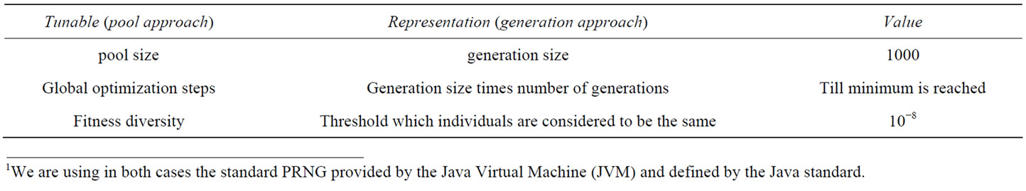
Table 1. Tunables in the pool algorithm and their values during the benchmark.
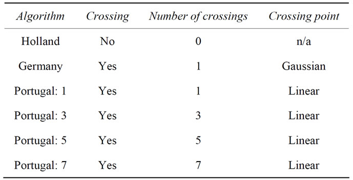
Table 2. Definition of the used algorithms.
Mating is accomplished by choosing two parents from the genetic pool. The mother is chosen purely randomly, whilst the father is chosen based on a fitness criterion. All structures in the pool are ranked by their fitness, a Gaussian distributed random number shaped with the factor 0.1 is chosen with its absolute value mapped to the rank in the pool.
If a local optimization step is carried out, it is a standard L-BFGS, as described in Ref. [21,22] and implemented in RISO [23], with very tight convergence criteria (e.g. 10−8 in fitness). The needed gradients are analytical in all cases.
Once the crossing, mutation and (if applicable) local optimization steps have been carried out on both children, only the fitter one will be returned to the pool. This fitter child will actually be added to the pool if it has a lower function value than the individual with the highest function value in the pool and does not violate the fitness diversity criterion. The fitness diversity is a measure to avoid premature convergence of the pool. Additionally, it promotes exploration by maintaining a minimum level of search space diversity, indirectly controlled via fitness values. For example, by assuming that two individuals with the same fitness (within a threshold) are the same, it eliminates duplicates. Since the pool size stays constant, the worst individual will be dropped automatically, keeping the pool dynamically updated.
For the benchmarking, we do not measure timings since they are of course dependent upon convergence criteria of the local optimization and potentially even on the exact algorithm used for the local optimization (e.g. L-BFGS vs. BFGS vs. CG). Therefore, our benchmarking procedure measures the number of global optimization steps where a step is defined to consist of mating, crossing, mutation and (if applicable) local optimization. The second difficulty is to define when the global optimum is found. We are using the function value as a criterion, trying to minimize the amount of bias one introduces by any measure.
It should be explicitly noted here that within the benchmarking of a given test function, this value stays constant in all dimensionalities which should in principle increase the difficulty with higher dimensionalities, again minimizing the amount of (positive) bias introduced. For all local tests with local optimization enabled, five independent runs have been carried out and a standard deviation is given.
3. Standard Benchmark Functions
Any approach towards global optimization should be validated with a set of published benchmark functions and/or problems. In the area of benchmark functions a broad range of published test functions exists, designed to stress different parts of a global optimization algorithm. Among the most popular ones are Schwefel’s, Rastrigin’s, Ackley’s, Schaffer’s F7 and Schaffer’s F6 functions. They have the strength of an analytical expression with a known global minimum and, in the case of all but the last function, they are extendable to arbitrary dimensionality allowing for scaling investigations. Contrary to assumptions made frequently, however, most of these benchmark functions do not allow to discriminate between algorithmic variations in the global optimization, nor do they give a true impression of the difficulty to be expected in real-life applications, as we will demonstrate in the following subsections.
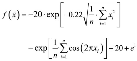
3.1. Ackley’s Function
Ackley's function has been first published in Ref. [24] and has been extended to arbitrary dimensionality in Ref. [25]. It is of the form
 (1)
(1)
with the global minimum at xi = 0.0. We considered this to be a relatively trivial function due to its shape consisting of a single funnel (see Figure 1). Nevertheless, this function type potentially has relevance for real-world applications since, e.g., the free energy hypersurface of proteins is considered to be of similar, yet less symmetric, shape.
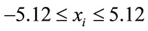
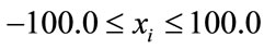
The initial randomized points were drawn from the interval
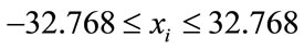 (2)
(2)
for all xi, which is to our knowledge the normal benchmark procedure for this function.
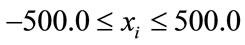
As can be seen from Figure 2, without local optimization steps the choice of genotype operator makes almost no difference; all cases exhibit excellent linear scaling. The only deviating case is the mutation-only algorithm, Holland, which has a higher prefactor in comparison to
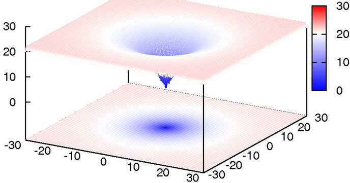
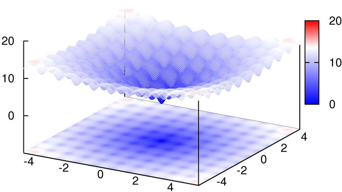
Figure 1. 2D-plot of Ackley’s Function, full search space (top) and fine structure (bottom).
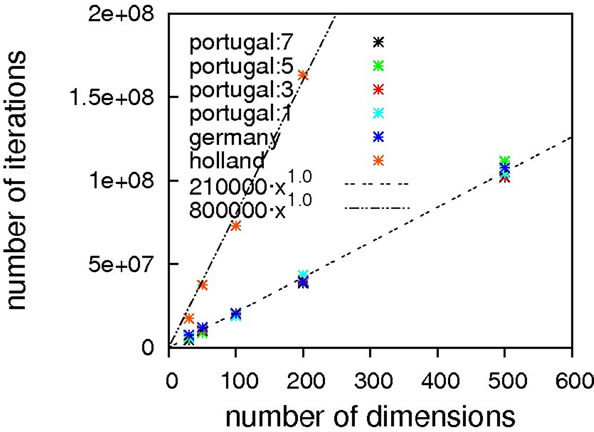
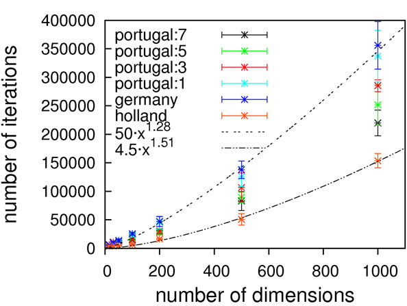
Figure 2. Scaling results for Ackley’s function, without (top) and with local optimization (bottom).
the other algorithms but still exhibits the same (linear) scaling. With local optimization enabled, the results do vary more. Results up to 500 dimensions do not allow for a concise statement on the superiority of a specific crossover operator. We therefore extended the benchmarking range up to one thousand dimensions, hoping for a clearer picture. It should be noted here that on a standard contemporary 24-core compute node, these calculations took 3.5 minutes on average (openJDK7 on an openSUSE 11.4), demonstrating the good performance of our framework.
Still, these results obviously allow for the conclusion that Ackley’s benchmark function should be considered to be of trivial difficulty since linear scaling is achievable already without local optimization. Any state-of-the-art global optimization algorithm should be capable of solving it with a scaling close to linear.
Also, we want to demonstrate an interesting aspect of Ackley’s benchmark function when manipulating the analytical gradient expression in a distinct manner. In general the modification of gradients in order to simplify the problem is not unheard of in applications of global optimization techniques to chemical problems (see e.g. Ref. [26]) and we therefore consider it to be of interest. The analytical gradient for a gradient element i is defined as
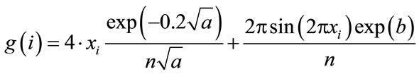 (3)
(3)
with
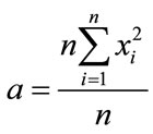 (4)
(4)
and
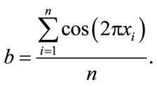 (5)
(5)
The simple modification that
 (6)
(6)
and
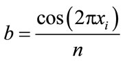 (7)
(7)
does not only drastically simplify the gradient expression, but also further helps to simplify the global optimization problem. As can be seen in Figure 3, this simplification effectively decouples the dimensions, thereby smoothing the search space.
With this simplification in place, Ackley’s function can be solved by simply locally optimizing a couple of randomized individuals (the first step of our global opti-
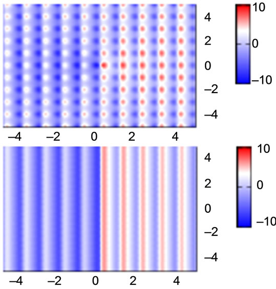
Figure 3. Contour plots of gradient element ×1 of a 2D Ackley’s Function, exact (top) and simplified (bottom).
mization algorithms) up to 10000 dimensions with constant effort (see Figure 4).
3.2. Rastrigin’s Function
Rastrigin’s function [27,28] does have fewer minima within the defined search space of
 (8)
(8)
but its overall shape is flatter than Ackley’s function which should complicate the general convergence towards the global optimum at xi = 0.0.
We defined Rastrigin’s function (Figure 5) with an additional harmonic potential outside the search space to force the solution to stay within those boundaries when using unrestricted local optimization steps.
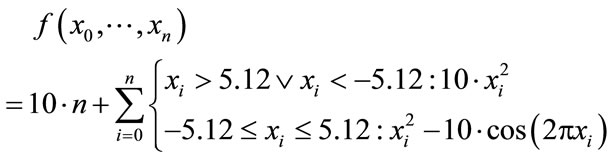 (9)
(9)
As can be seen from Figure 6, the scaling is excellent with all tested crossing operators; Holland again being the easily rationalizable exception, in the case without local optimization. In the case with local optimization, a contrasting picture can be seen.
The scaling once more does not deviate much between the different algorithms with the prefactor making the major difference. Interestingly, by far the best prefactor and scaling is obtained with Holland. Probably, the rather non-intrusive behaviour of a mutation-only operator fits this problem best since it provides a better short-range exploration than any of the crossing algorithms. We assume the rather high number of global optimization steps (also in comparison to the non-locopt case) to be due to a repeated finding of the same, non-
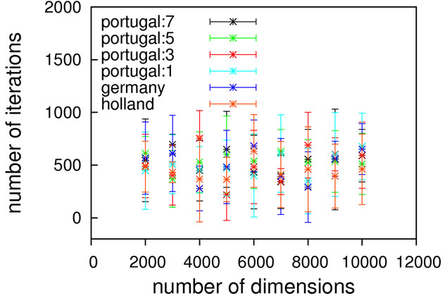
Figure 4. Scaling behavior of Ackley’s function with a modified gradient expression.
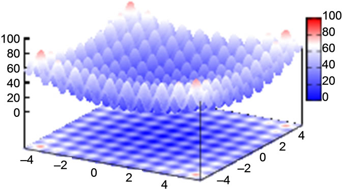
Figure 5. 2D plot of Rastrigin’s function.
optimal minima. Inclusion of taboo-search features [29] into the algorithm might be of help for real-world problems of such a type, not reducing the number of global optimization steps but the amount of time spent in local optimizations rediscovering already known minima.
Just as Ackley’s function discussed earlier, it is possible to conclude that Rastrigin’s function should be solvable with almost linear scaling using contemporary algorithms.
3.3. Schwefel’s Function
In comparision to Rastrigin’s function, Schwefel’s function [30] (Figure 7) adds the difficulty of being less symmetric and having the global minimum at the edge of the search space
 (10)
(10)
at position xi = 420.9687. Additionally, there is no overall, guiding slope towards the global minimum like in Ackley’s, or less extreme, in Rastrigin’s function.
Again, we added a harmonic potential around the search space
 (11)
(11)
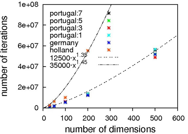
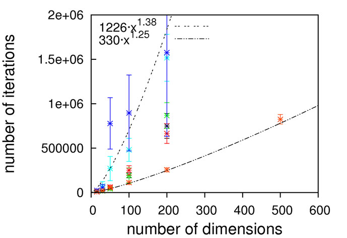
Figure 6. Scaling results for Rastrigin’s function; without local optimization (top), with local optimization (middle) and zoom with local optimization (bottom).
Figure 7. 2D plot of Schwefel’s function.
since otherwise our unrestricted local optimization finds lower-lying minima outside the principal borders. As can be seen from Figure 8, sub-quadratic scaling can be achieved with and without local optimization. Once more, without local optimization the non-crossing algorithm has a higher prefactor but the same scaling as the others, which is equalized when turning on local optimizations. In this particular case, the usage of local optimization steps has the potential to slightly affect the scaling from 1.15 to 1.75.
Again, we must come to the conclusion that a subquadratic scaling is far better than what we would expect to obtain for real-world problems, restricting the usage of Schwefel’s function as a test-case for algorithms designed to solve the latter.
3.4. Schaffer’s F7 Function
Schaffer’s F7 function is defined as
 (12)
(12)
with
 (13)
(13)
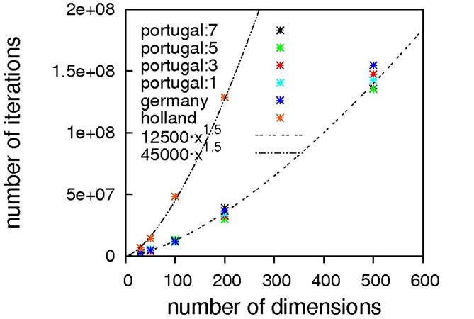
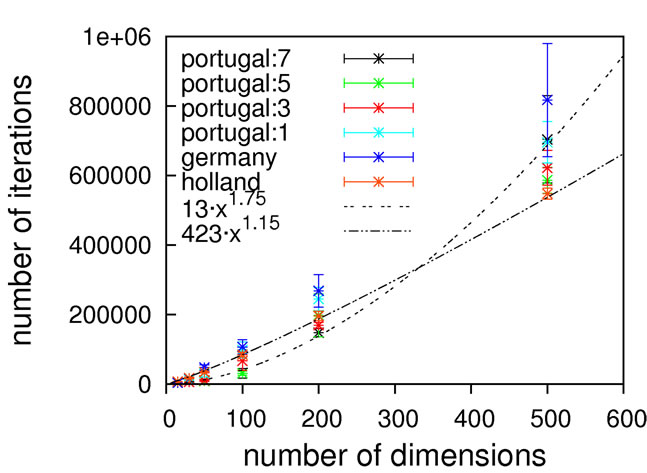
Figure 8. Scaling results for Schwefel’s function, without (top) and with local optimization (bottom).
in n-dimensional space within the boundaries
 (14)
(14)
As can be seen from Figure 9, concentric barriers need to be overcome to reach the global minimum xi = 0.0.
Judging from the results depicted in Figure 10, this function is capable of discriminating between different algorithmic implementations. For the Gaussian-based single point crossover (germany) the scaling is quartic, while all the other algorithms are scaling linearly with the problem size. The sublinear scaling is an artifact of the high ratio of crossover cuts (up to seven) to problem size (only 40D) and it can be expected to increase to linear for higher dimensionalities. Interestingly, the performance of the mutation-only algorithm again is on par with the algorithms employing crossover operators. We see such a bias with all the benchmark functions so far, and this does not conform to our experience with real-life problems. Therefore, conclusions on the importance of mutation for global optimization may be too positive when based on an analysis using only these functions.
Nevertheless, we consider Schaffer’s F7 function the most interesting of the benchmark functions studied so far. It should be explicitly noted though that a forty-dimensional problem size will definitely be too small when exclusively analyzing algorithms employing multiple crossover cuts.
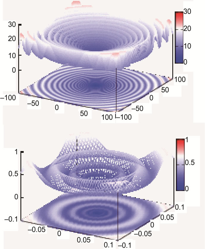
Figure 9. Schaffer’s F7 function, full search space (top) and fine structure (bottom).
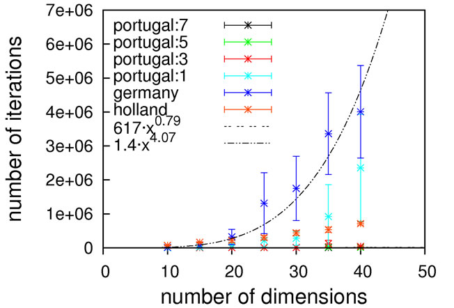
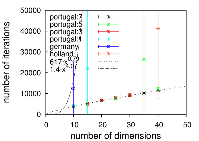
Figure 10. Scaling results for Schaffer’s F7 function, with local optimization.
3.5. Schaffer’s F6 Function
For completeness, we would like to present some nonscaling results using Schaffer’s F6 function as a benchmark:
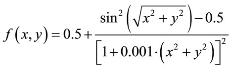 (15)
(15)
As can be seen in Figure 11, the difficulty in this function is that the size of the potential maxima that need to be overcome to get to a minimum increases the closer one gets to the global minimum.
In Table 3, results can be found which were obtained with Holland and with the one-point crossover operators (obviously, with a real-number encoded genotype approach, not more cuts can take place for a two-dimensional function). The results are outcomes of three successive runs which is sufficient to obtain a general picture of the trend.
The difference between the Portugal and Germany approach in this very special case is that Germany in contrast to Portugal can also yield a crossover point before the first number, effectively reducing it to a partial non-crossing approach.
Interestingly, we do see converse tendencies between
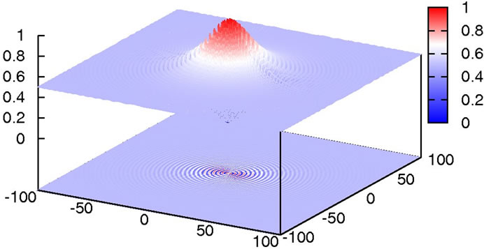
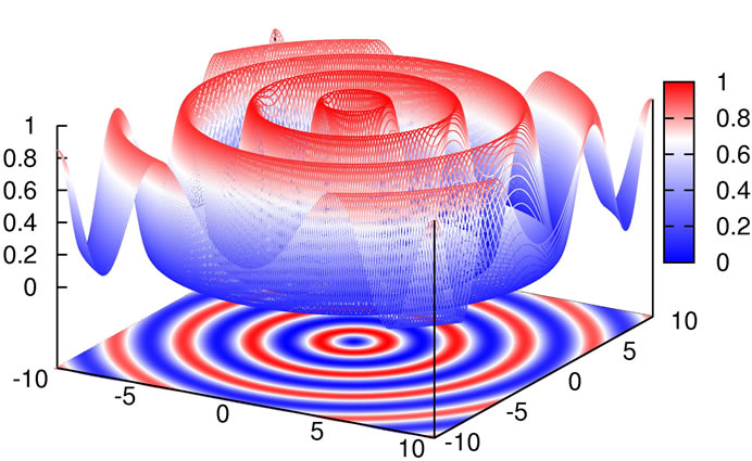
Figure 11. Plot of Schaffer’s F6 function.
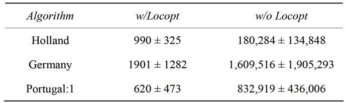
Table 3. Different results for Schaffer’s F6 function with one-point and zero-point crossover operators.
the case with and without local optimization. We see a clear preference of the Germany crossover operator over Portugal without local optimization. Taking the results of the non-crossing operator into account, it seems clear that without local optimization too much crossing is harmful in terms of convergence to the global minimum. With local optimization enabled, these differences disappear, sometimes even allowing the global minimum to be found in the initial (and therefore never crossed) pool of solutions.
Although Schaffer’s function shows an impressive difficulty for a two-dimensional function, it should still be easily solvable with and without local optimization.
3.6. Scatter of the Benchmarking Results
Obviously any stochastic approach is difficult to benchmark in a reliable manner. Therefore, we would like to discuss the scatter of the benchmarking results. We will try to approximate possible deviations for every crossover operator used with and without local optimization for a two hundred dimensional Ackley’s function. For this, we present in Table 4 results from ten runs per crossover operator used.
Of course, the results do not and cannot take all or the maximum possible deviations into account since in principle there should be a probability distribution from a single iteration up to infinity which can only be captured adequately by an infinite amount of successive runs. Nevertheless, ten successive runs can be considered to give a rough idea of the location of the maximum.
The impression gained in the previous sections, namely that the exact nature of the genotype operator does not seem to make a difference when using local optimization, holds true also with enhanced statistics for this case. Similarly, the differences seen in the runs without local optimizations between the crossing operators and the non-crossing operator, Holland, remain also when averaging over more runs.
This allows for the conclusion that the results presented in the previous sections are giving a reasonably accurate picture, despite of course suffering from the inherent uncertainty in all stochastic methods which cannot be circumvented.
Upon closer examination of the data in Table 4, some seemingly systematic trends can be observed, calling for speculative explanations. A general tendency observed is the reduced spread when local optimization is turned off, probably because a higher diversity can be maintained providing a better and more reliable convergence. Another tendency is the reduced spread when more—or no—crossover points are used. In the case of more crossover points this can be explained with more crossover points causing bigger changes in each step; this improves search space coverage, which in turn makes the runs more reproducible. For the reduced scatter of the non-crossing
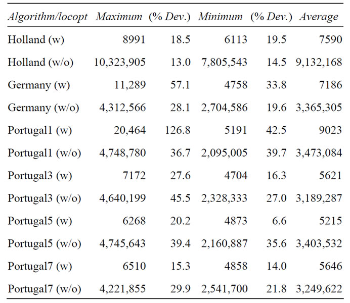
Table 4. Different results for Schaffer’s F6 function with one-point and zero-point crossover operators.
operator, the explanation is obviously the opposite, since this operator minimizes changes to the genome, allowing for a better close-range exploration.
Despite of these interesting observations, we refrain from further analysis since this would lead us outside of the scope of the present article.
4. Gaussian Benchmark Class
To our experience from the global optimization of chemical systems, real-world problems are considerably more challenging than the benchmark functions described above. For example, in the case of the relatively trivial Lennard-Jones (LJ) clusters, the best scaling we could reach is cubic [8]. Therefore, we feel a need for benchmarks with a difficulty more closely resembling real-world problems.
Defining new benchmark functions is of course not trivial since they should fulfill certain criteria.
1. Not trivial to solve
2. Easy to extend to higher dimensions, causing higher difficulty
3. Possibility to define an analytical gradient, for gradient-based methods
4. Of multimodal nature, with a single, well-defined global minimum.
To have better control over these criteria when generating benchmark functions, a few “search landscape generators” have been proposed in recent years [31-33]. The simplest and most flexible of these is the one based on randomly distributed Gaussians [31]. For convenience, we have used our own implementation of this concept, abbreviated GRUNGE (GRUNGE: Randomized, UNcorrelated Gaussian Extrema), defined and discussed in the following. We would like to emphasize already at this point that our intention in using GRUNGE is not to re-iterate known results from Ref. [31] and similar work, but to directly contrast the OGOLEM behavior displayed in section III with its different behavior in the GRUNGE benchmark. This shows strikingly that the rather uniform results in section III are not a feature of OGOLEM but rather a defect of that benchmark function class.
We define a function as a set of randomized Gaussians
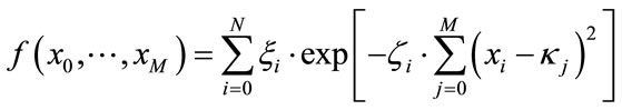 (16)
(16)
with the random numbers ξi, ζi and κi being the weight, width and position of the i-th Gaussian in M-dimensional space. As can be easily seen, this class of benchmarking problems provides (besides the search space size) two degrees of freedom. One is the number N of randomized Gaussians in the search space and M being the dimensionality of the Gaussians2. More subtly, there is also a connection between these two characteristics and the Gaussian widths within the maximal coordinate interval (i.e. the Gaussian density). With proper choices of these numbers, one can smoothly tune such a benchmark function between the two extremes of a “mountain range” (many overlapping Gaussians) and a “golf course” (isolated Gaussians with large flat patches in-between).
Functions in this class of benchmarks are not easy to solve, easily extendable in dimensionality and—through the use of Gaussians—the definition of an analytical gradient is trivial. The only problem remaining is to predetermine the position and depth of the global minimum. Here, other benchmark function generators like, e.g. the polynomial ones proposed by Gaviano et al. [33] and Locatelli et al. [32], allow for more control, but at the price of more uniform overall features of the generated test functions, which is exactly what we want to avoid. We also do not want to enforce a known global minimum by introducing a single, dominating Gaussian with excessively large weight by hand. Thus, the only remaining possibility is to define a fine grid over the search space and to run local optimizations starting at every grid point, to obtain a complete enumeration of all minima within the search space. Due to the simple functional form and to the availability of an analytical gradient, this is a realistic proposition for moderately-dimensioned examples (10D) containing a sufficiently great number of sufficiently wide Gaussians. In contrast to the traditional benchmarks examined in the previous sections, the GRUNGE function is not deliberately designed to be deceptive, in any number of dimensions. Instead, due to the heavy use of random numbers in its definition, it does not contain any correlations whatsoever. To our experience, this feature makes GRUNGE benchmarks much harder than any of the traditional benchmarks. We cannot offer formal proofs at this stage, but our distinct impression from many years of global optimization experience is that realistic problems tend to fall in-between these two extremes, being harder than traditional benchmarks but less difficult (less uncorrelated) than GRUNGE.
Obviously, a full exploration of the randomize Gaussians set of benchmark functions requires an exclusive and extensive study, which has already been started by others [31]. As already mentioned above, our sole intention here is to provide a contrast to the OGOLEM behavior noted in section 3. To this end, we present results based on solving a ten-dimensional GRUNGE benchmark with 2000 gaussians (GRUNGE[10,2000]) within a search space of
 (17)
(17)
with local optimization enabled.
As can be seen from the results in Table 5, the average
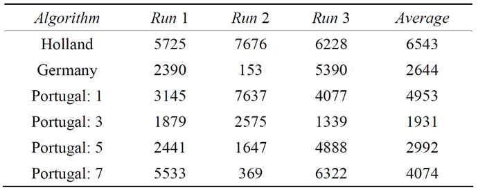
Table 5. GRUNGE[10,2000] benchmarking results with local optimization steps.
of three independent runs of all algorithms yields results within the same order of magnitude. When comparing the numbers in Table 5 with the results given above for the conventional benchmark functions, e.g. with those in Table 4, one should remember the differences in dimensionality: Here we are dealing with a 10-dimensional problem with 2000 minima, whereas in Table 4 we reported the performance on the 200-dimensional Ackley function with the number of minima being several orders of magnitude higher. This gives an indication of what we experience as a big difference in difficulty.
It should be noted, however, that in two cases the global optimum could be found within the locally optimized initial parameter sets. While this demonstrates once more that a randomly distributed initial parameter set can have an extraordinary fitness, it also indicates that higher dimensional GRUNGE benchmarks are necessary to better emulate real-world problems.
We also did some tests without local optimization, showing that the GRUNGE benchmark with our randomly generated Gaussians is extremely difficult to solve without local optimization, requiring almost 19 million global optimization steps with Portugal: 3. We suspect that this level of difficulty is related to inherent features of the GRUNGE benchmark (e.g. to the completely missing correlation between the locations and depths of the minima) but also to features of the specific GRUNGE[10,2000] incarnation used here (i.e. this particular Gaussian distribution and density), but decide to leave this sidetrack at this point.
5. Lunacek’s Function
Lunacek’s function [34], also known as the bior double-Rastrigin function, is a hybrid function consisting of a Rastrigin and a double-sphere part and is designed to model the double-funnel character of some difficult LJ cases, in particular LJ38.
 (18)
(18)
 (19)
(19)
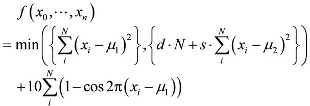
This indicates that there is an interest in developing benchmark functions of higher difficulty, and indeed the developed function provides an interesting level of difficulty, as we show below. Nevertheless, we would like to dispute the notion that it resembles certain real-world problems and the source of their difficulty. Specifically, Lunacek et al. claim that the global optimization of homogeneous LJ clusters is one of the most important applications of global optimization in the field of computational chemistry. Furthermore, they claim that the most difficult instances of the LJ problem possess a double-funnel landscape. The former claim is a rather biased view and promotes the importance of homogenous LJ clusters from a mere benchmark system to a hot-spot of current research. As the broad literature on global cluster structure optimization documents (cf. Reviews [11,35-37] and references cited therein), current challenges in this field rather are directed towards additional complications in real-life applications, e.g. how to taylor search steps to dual-level challenges of intraand intermolecular conformational search in clusters of flexible molecules, or how to reconcile the vast number of necessary function evaluations with their excessive cost at the ab-initio quantum chemistry level. In terms of search difficulty, the homogeneous LJ case is now recognized as rather easy for most cluster sizes, interspersed with a few more challenging problem realizations at certain sizes, with LJ38 being the smallest and hence the simplest of them. This connects to the second claim by Lunacek et al., namely that the difficulty of LJ38 arises from the double-funnel shape of its search landscape, which is captured by their test function design. It is indeed tempting to conclude from the disconnectivity graph analysis by Doye, Miller and Wales [38] that there are two funnels, a narrow one containing the fcc global minimum, separated by a high barrier from the broad but less deep one containing all the icosahedral minima. Even if this were true (to our knowledge, such a neat separation of the two structural types in search space has not been shown), it would give rise to only two funnels in a 108-dimensional search space, which is not necessarily an overwhelming challenge and also not quite the same as what Equation 18 offers. Lunacek’s function is specifically designed to poison global optimization strategies working with bigger population sizes. This is achieved through the double sphere contribution which constructs in every dimension a fake minimum, e.g. when using the settings s = 0.7, d = 1.0, with the optimal minimum located at xi = 2.5. As Lunacek et al. have proven in their initial publication, the function is very efficient in doing this. This is an observation that we can support from some tests on 30-dimensional cases.
Clearly, this is a markedly different behavior than that observed above for Ackley’s, Rastrigin’s, Schwefel’s or Schaffer’s functions, coming closer to what we experienced in tough application cases. Therefore, it is not surprising that additional measures developed there are also of some help here. One possibility is to adopt a niching strategy, similar to what was applied to reduce the solution expense for the tough cases of homogenous LJ clusters to that of the simpler ones [8]. In essence, this ensures a minimum amount of diversity in the population, preventing premature collapse into a non-globally optimal solution.
The most trivial implementation of niching is to employ a static grid over search space and to allow only a certain maximal population per grid cell (MNIC, maximum number of individuals per grid cell). Already this trivial change allows the previously unsolvable function to be solved in 30 dimensions, as can be seen from Table 6. Solving higher dimensionalities (e.g. 100D) with this approach suffers again from dimensionality explosion, this time in the number of grid cells. Additionally, such a basic implementation truncates the exploitation abilities of the global optimization algorithm. This causes the algorithm with static niches to require more steps in those low dimensional cases where the problem can also be solved without. From our experience with LJ clusters, we expect more advanced niching strategies, for example dynamic grids, to prove useful with higher dimensionalities and render the function even less difficult.
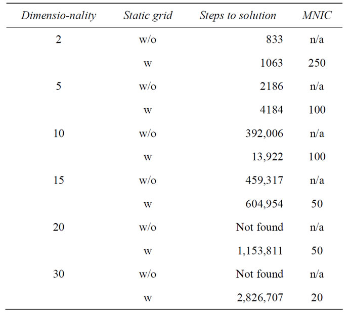
Table 6. Exemplary benchmarking results of the Lunacek function. All results obtained with local optimization and the germany algorithm. Not found corresponds to more than 10 million unsuccessful global optimization steps. MNIC is the maximum number of individuals allowed per grid cell.
As it seems to be common wisdom in this area, applications do contain some degree of deceptiveness and different degrees of minima correlation, as well as different landscape characteristics, sampling all possibilities between golf courses and funnels. All of that can be captured with the GRUNGE setup. It thus offers all the necessary flexibility and simplicity, combined in a single function definition. The obvious downsides are the absence of a pre-defined global minimum (which can also be interpreted as a guarantee for avoiding biases towards it) and the need to tune many parameters to achieve a desired landscape shape.
6. Summary and Outlook
Scaling investigations for four different, standard benchmark functions have been presented, supplemented by performance tests on a fifth function. Using straightforward GA techniques without problem-specific ingredients, the behavior we observe in all these cases is markedly different from what we observe upon applying the same techniques to real-world problems (often including system-specific additions): All benchmarks but one can be solved with sub-quadratic scaling, whereas in real-world applications we can get cubic scaling at best and often have to settle for much worse. In addition, the benchmarks often do not allow for statistically significant conclusions regarding the performance of different crossover operators, nor for a decision on whether to include local optimization or not. Thus, overall, benchmarks of this type do not seem to fulfill their purpose of test beds with relevance for practical applications in global cluster structure optimization or similar areas.
We have contrasted the behavior on those traditional benchmark functions with that on two different types of functions. One type is the “landscape generator” class, shown here in a particularly simple realization, namely search landscapes generated by randomly distributed Gaussians. Varying Gaussian characteristics (depth, width, density, dimensionality), search space features can be tuned at will, on the full scale between a “mountain range” and a “golf course”. In addition, since the constituting Gaussians are completely uncorrelated, the difficulty of this problem class is inherently larger than that of the traditional benchmark functions where the minima characteristics follow a simple rule by construction. This is strikingly reflected in our tests results on this benchmark class.
As yet another class of benchmark functions we have shown the deceptive type, designed to lead global optimization astray. Their difficulty can be diminished significantly by making the global search more sophisticated, in the case of population-based searches by ensuring a sufficient degree of diversity in the population. Given a sufficiently flexible setup, this benchmark class merely is a subclass of the landscape generators.
Further work will be required to confirm our suspicion that real-world problems often fall in-between the traditional, rather simple benchmark functions on the one hand and the less correlated, more deceptive ones on the other hand, both with respect to their search space characteristics and to the difficulty they present for global optimization algorithms. In any case, we hope to have shown convincingly that due to their simplicity functions from the traditional benchmark functions should not be used on their own, neither to aid global optimization algorithm development nor to judge performance.
REFERENCES
- A. B. Ozer, “A Multilingual Ontology Framework for R&D Project Management Systems,” Expert Systems with Applications, Vol. 37, No. 6, 2010, pp. 4632-4631.
- R. Thangaraja, M. Panta and A. Abraham, “New Mutation Schemes for Differential Evolution Algorithm and Their Application to the Optimization of Directional Over-Current Relay Settings,” Applied Mathematics and Computation, Vol. 216, No. 2, 2010, pp. 532-544. doi:10.1016/j.amc.2010.01.071
- M. J. Hirsch, P. M. Pardalos and M. G. C. Resende, “Speeding up Continuous GRASP,” European Journal of Operational Research, Vol. 205, No. 3, 2010, pp. 507- 521. doi:10.1016/j.ejor.2010.02.009
- L. Zhao, F. Qian, Y. Yang, Y. Zeng and H. Su, “Automatically Extracting T-S Fuzzy Models Using Cooperative Random Learning Particle Swarm Optimization,” Applied Soft Computing, Vol. 10, No. 3, 2010, pp. 938- 944. doi:10.1016/j.asoc.2009.10.012
- Q.-K. Pan, P. N. Suganthan, M. F. Tasgetiren and J. J. Liang, “A Self-Adapting Global Best Harmony Search Algorithm for Continuous Optimization Problems,” Applied Mathematics and Computation, Vol. 216, No. 3, 2010, pp. 830-848. doi:10.1016/j.amc.2010.01.088
- “Black Box Optimization Benchmarking,” 2012. http://coco.gforge.inria.fr/
- B. Hartke, “Global Geometry Optimization of Clusters Using Genetic Algorithms,” The Journal of Physical Chemistry, Vol. 97, No. 39, 1993, pp. 9973-9976. doi:10.1021/j100141a013
- B. Hartke, “Global Cluster Geometry Optimization by a Phenotype Algorithm with Niches,” Journal of Computational Chemistry, Vol. 20, No. 16, 1999, pp. 1752-1759. doi:10.1002/(SICI)1096-987X(199912)20:16<1752::AID-JCC7>3.0.CO;2-0
- B. Hartke, “Global Geometry Optimization of Molecular Clusters: TIP4P Water,” Zeitschrift für Physikalische Chemie, Vol. 214, No. 9, 2000, pp. 1251-1264. doi:10.1524/zpch.2000.214.9.1251
- B. Bandow and B. Hartke, “Larger Water Clusters with Edges and Corners on Their Way to Ice,” The Journal of Physical Chemistry A, Vol. 110, No. 17, 2006, pp. 5809- 5822. doi:10.1021/jp060512l
- J. M. Dieterich and B. Hartke, “OGOLEM: Global Cluster Structure Optimisation for Arbitrary Mixtures of Flexible Molecules,” Molecular Physics, Vol. 108, No. 3-4, 2010, pp. 279-291. doi:10.1080/00268970903446756
- J. M. Dieterich and B. Hartke, “Composition-Induced Structural Transitions in Mixed Lennard-Jones Clusters,” Journal of Computational Chemistry, Vol. 32, No. 7, 2011, pp. 1377-1385. doi:10.1002/jcc.21721
- D. Whitley, S. Rana, J. Dzubera and K. E. Mathias, “Evaluating Evolutionary Algorithms,” Artificial Intelligence, Vol. 85, No. 1-2, 1996, pp. 245-276. doi:10.1016/0004-3702(95)00124-7
- L. T. Wille and J. Vennik, “Computational Complexity of the Ground-State Determination of Atomic Clusters,” Journal of Physics A: Mathematical and General, Vol. 18, No. 8, 1985, pp. 419-422. doi:10.1088/0305-4470/18/8/003
- G. W. Greenwood, “Revisiting the Complexity of Finding Globally Minimum Energy Configurations in Atomic Clusters,” Zeitschrift für Physikalische Chemie, Vol. 211, No. 1, 1999, pp. 105-114. doi:10.1524/zpch.1999.211.Part_1.105
- R. Salomon, “Re-Evaluating Genetic Algorithm Performance under Coordinate Rotation of Benchmark Functions,” Biosystems, Vol. 39, No. 3, 1996, pp. 263-278. doi:10.1016/0303-2647(96)01621-8
- H. Takeuchi, “Clever and Efficient Method for Searching Optimal Geometries of Lennard-Jones Clusters,” Journal of Chemical Information and Modeling, Vol. 46, No. 5, 2006, pp. 2066-2070. doi:10.1021/ci600206k
- H. Takeuchi, “Development of an Efficient Geometry Optimization Method for Water Clusters,” Journal of Chemical Information and Modeling, Vol. 48, No. 11, 2008, pp. 2226-2233. doi:10.1021/ci800238w
- R. L. Johnston, “Atomic and Molecular Clusters,” Taylor & Francis, London, 2002. doi:10.1201/9781420055771
- D. E. Goldberg, “Genetic Algorithms in Search, Optimization and Machine Learning,” Addison-Wesley, Boston, 1989.
- J. Nocedal, “Updating Quasi-Newton Matrices with Limited Storage,” Mathematics of Computation, Vol. 35, No. 151, 1980, pp. 773-782. doi:10.1090/S0025-5718-1980-0572855-7
- H. Matthies and G. Strang, “The Solution of Nonlinear Finite Element Equations,” International Journal for Numerical Methods in Engineering, Vol. 14, No. 11, 1979, pp. 1613-1626. doi:10.1002/nme.1620141104
- R. Dodier, “RISO: An Implementation of Distributed Belief Networks in Java,” 2012. http://riso.sourceforge.net
- D. H. Ackley, “A Connectionist Machine for Genetic Hillclimbing,” Kluwer Academic Publishers, Dordrecht, 1987. doi:10.1007/978-1-4613-1997-9
- T. Bäck, “Evolutionary Algorithms in Theory and Practice,” Oxford University Press, Oxford, 1996.
- G. Rauhut and B. Hartke, “Modeling of High-Order Many-Mode Terms in the Expansion of Multidimensional Potential Energy Surfaces,” Journal of Chemical Physics, Vol. 131, No. 1, 2009, pp. 014108-014121. doi:10.1063/1.3160668
- A. Törn and A. Zilinskas, “Global Optimization, Lecture Notes in Computer Science No. 350,” Springer Verlag, Berlin, 1980.
- H. Mühlenbein, D. Schomisch and J. Born, “The Parallel Genetic Algorithm as Function Optimizer,” Parallel Computing, Vol. 17, No. 6-7, 1991, pp. 619-632. doi:10.1016/S0167-8191(05)80052-3
- S. Stepanenko and B. Engels, “Tabu Search Based Strategies for Conformational Search,” The Journal of Physical Chemistry A, Vol. 113, No. 43, 2009, pp. 11699-11705. doi:10.1021/jp9028084
- H.-P. Schwefel, “Numerical Optimization of Computer Models,” Wiley, Chinchester, 1981.
- M. Gallagher and B. Yuan, “A General-Purpose Tunable Landscape Generator,” IEEE Transactions on Evolutionary Computation, Vol. 10, No. 5, 2006, pp. 590-603. doi:10.1109/TEVC.2005.863628
- B. Addis and M. Locatelli, “A new class of Test Functions for Global Optimization,” Journal of Global Optimization, Vol. 38, No. 3, 2007, pp. 479-501. doi:10.1007/s10898-006-9099-8
- M. Gaviano, D. E. Kvasov, D. Lera and Y. D. Sergeyev, “Algorithm 829: Software for Generation of Classes of Test Functions with Known Local and Global Minima for Global Optimization,” ACM Transactions on Mathematical Software, Vol. 29, No. 4, 2003, pp. 469-480. doi:10.1145/962437.962444
- M. Lunacek, D. Whitley and A. Sutton, “The Impact of Global Structure on Search,” In: G. Rudolph, T. Jansen, S. Lucas, C. Poloni and N. Beume, Eds., Parallel Problem Solving from Nature, Springer Verlag, Berlin, 2008, pp. 498-507.
- B. Hartke, “Structural Transitions in Clusters,” Angewandte Chemie International Edition, Vol. 41, No. 9, 2002, pp. 1468-1487. doi:10.1002/1521-3773(20020503)41:9<1468::AID-ANIE1468>3.0.CO;2-K
- B. Hartke, “Application of Evolutionary Algorithms to Global Cluster Geometry Optimization,” Structure and Bonding, Vol. 110, 2004, pp. 33-53. doi:10.1007/b13932
- B. Hartke, “Global Optimization,” Wiley Interdisciplinary Reviews: Computational Molecular Science, Vol. 1, No. 6, 2011, pp. 879-887. doi:10.1002/wcms.70
- J. P. K. Doye, M. A. Miller and D. J. Wales, “Evolution of the Potential Energy Surface with Size for Lennard-Jones Clusters,” Journal of Chemical Physics, Vol. 111, No. 18, 1999, pp. 8417-8428. doi:10.1063/1.480217
NOTES
1We are using in both cases the standard PRNG provided by the Java Virtual Machine (JVM) and defined by the Java standard.
2As a side note, we write GRUNGE[M,N], e.g. for 2000 gaussians in a ten dimensional space GRUNGE[10,2000].